from google.colab import drive
drive.mount("/content/drive")
Mounted at /content/drive
라이브러리 불러오기
아래 라이브러리들을 모두 암기하시기를 바랍니다.
import pandas as pd
import numpy as np
from sklearn.model_selection import train_test_split
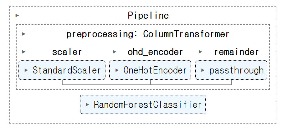
from sklearn.preprocessing import StandardScaler, OneHotEncoder
from sklearn.compose import ColumnTransformer
from sklearn.pipeline import Pipeline
## from sklearn.metrics import make_scorer, mean_squared_error## from sklearn.ensemble import RandomForestRegressorfrom sklearn.metrics import roc_auc_score
from sklearn.ensemble import RandomForestClassifier
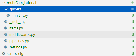
$ scrapy startproject multiCam_tutorial
New Scrapy project 'multiCam_tutorial', using template directory 'C:\Users\j2hoo\OneDrive\Desktop\your_project_folder\venv\Lib\site-packages\scrapy\templates\project', created in:
    C:\Users\j2hoo\OneDrive\Desktop\your_path\multiCam_tutorial

You can start your first spider with:
    cd multiCam_tutorial
    scrapy genspider example example.com
해당 multiCam_tutorial 경로에서 다음 명령어를 실행하여 타겟 사이트를 설정한다.
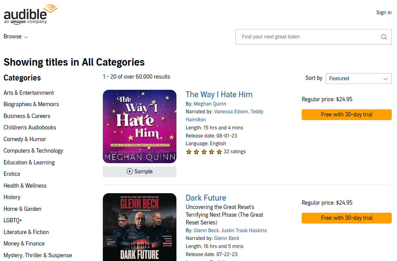
$ scrapy genspider audible www.audible.com/search
Created spider 'audible' using template 'basic' in module:
  multiCam_tutorial.spiders.audible
$ scrapy startproject multiCam_tutorial
New Scrapy project 'multiCam_tutorial', using template directory 'C:\Users\j2hoo\OneDrive\Desktop\your_project_folder\venv\Lib\site-packages\scrapy\templates\project', created in:
    C:\Users\j2hoo\OneDrive\Desktop\your_path\multiCam_tutorial

You can start your first spider with:
    cd multiCam_tutorial
    scrapy genspider example example.com
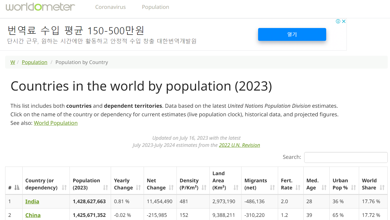
$ scrapy genspider worldometer www.worldometers.info/world-population/population-by-country
Created spider 'worldometer' using template 'basic' in module:
  multiCam_tutorial.spiders.worldometer
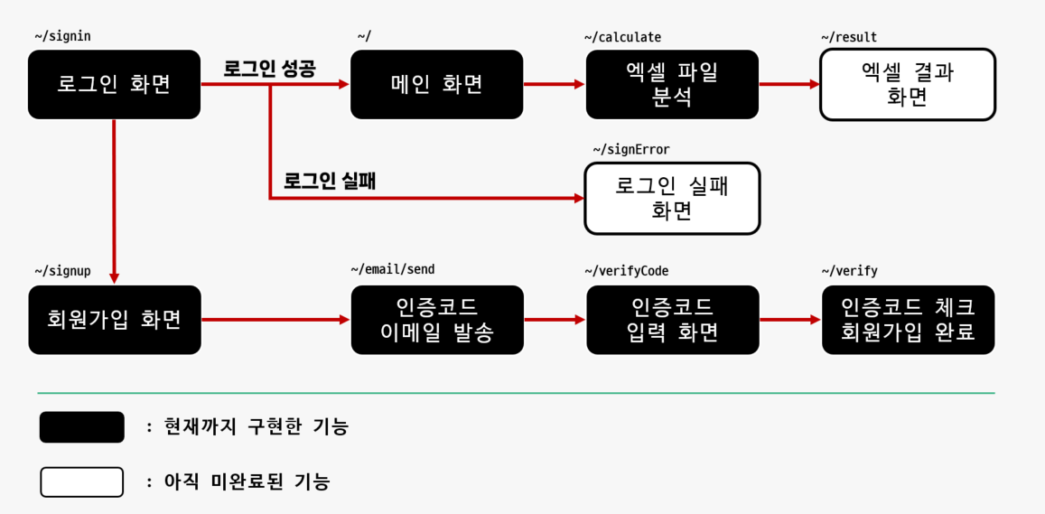
calculate/ 경로는 초기에 ExcelCalculate > ExcelCalculate > urls.py에서 이미 설정해놨다.
링크 참조 :
from django.contrib import admin
from django.urls import path, include

urlpatterns = [
    path('email/', include('sendEmail.urls'), name="email"),
    path('calculate/', include('calculate.urls'), name="calculate"),
    path('', include('main.urls'), name="main"),
    path("admin/", admin.site.urls),
]
ExcelCalcalculate > calculate > urls.py 에서도 이미 설정을 해놨다.
from django.urls import path
from . import views

urlpatterns = [
    path('', views.calculate, name="calculate_do"),
]
check - 2 : views.py 구현
파일 경로 : ExcelCalculate > calculate > views.py
이 때, request.POST가 아닌 request.FILES를 이용한다.
# Create your views here.defcalculate(request):
file = request.FILES['fileInput']
print("# 사용자가 등록한 파일의 이름: ", file)
return HttpResponse("calculate, calculate function!")
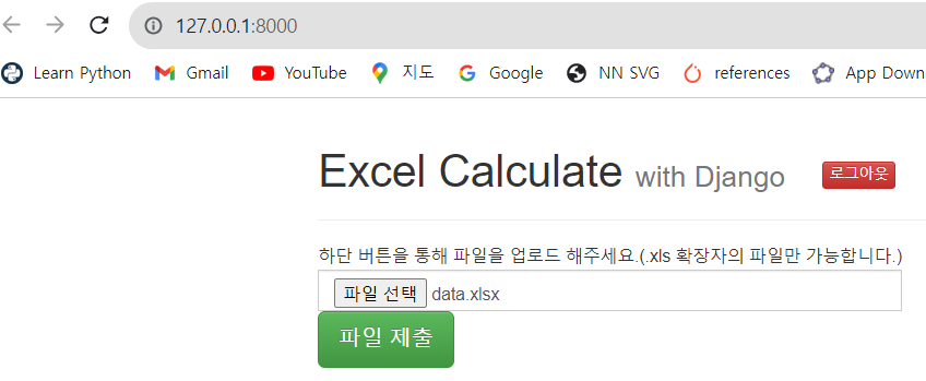
check - 3 : 테스트
이제 data.xlsx 파일을 업로드 한다.
파일 제출 버튼을 누를 시, 웹에서는 정상적으로 calculate, calculate function! 출력이 되어야 하고 터미널에서는 아래와 같이 print() 문구가 나와야 한다.