EDA with Housing Price Prediction - Handling Date
강의 홍보
- 취준생을 위한 강의를 제작하였습니다.
- 본 블로그를 통해서 강의를 수강하신 분은 게시글 제목과 링크를 수강하여 인프런 메시지를 통해 보내주시기를 바랍니다.
스타벅스 아이스 아메리카노를 선물로 보내드리겠습니다.
- [비전공자 대환영] 제로베이스도 쉽게 입문하는 파이썬 데이터 분석 - 캐글입문기

I. 개요
- 이제 본격적으로 Kaggle 데이터를 활용하여 분석을 진행한다.
- 데이터는 이미 다운 받은 상태를 전제로 하며, 만약에 데이터가 없다면 이전 포스팅에서 절차를 확인하기 바란다. (미리보기 가능)
II. 구글 드라이브 연동
- 구글 코랩을 시작하면 언제든지 가장 먼저 해야 하는 것은 드라이브 연동이다.
from google.colab import drive # 패키지 불러오기
from os.path import join

ROOT = "/content/drive"     # 드라이브 기본 경로
print(ROOT)                 # print content of ROOT (Optional)
drive.mount(ROOT)           # 드라이브 기본 경로 Mount

MY_GOOGLE_DRIVE_PATH = 'My Drive/Colab Notebooks/inflearn_kaggle/' # 프로젝트 경로
PROJECT_PATH = join(ROOT, MY_GOOGLE_DRIVE_PATH) # 프로젝트 경로
print(PROJECT_PATH)
/content/drive
Go to this URL in a browser: https://accounts.google.com/o/oauth2/auth?client_id=947318989803-6bn6qk8qdgf4n4g3pfee6491hc0brc4i.apps.googleusercontent.com&redirect_uri=urn%3aietf%3awg%3aoauth%3a2.0%3aoob&response_type=code&scope=email%20https%3a%2f%2fwww.googleapis.com%2fauth%2fdocs.test%20https%3a%2f%2fwww.googleapis.com%2fauth%2fdrive%20https%3a%2f%2fwww.googleapis.com%2fauth%2fdrive.photos.readonly%20https%3a%2f%2fwww.googleapis.com%2fauth%2fpeopleapi.readonly

Enter your authorization code:
··········
Mounted at /content/drive
/content/drive/My Drive/Colab Notebooks/inflearn_kaggle/
%cd "{PROJECT_PATH}"
/content/drive/My Drive/Colab Notebooks/inflearn_kaggle
- 위 코드가 에러 없이 돌아간다면 이제 데이터를 불러올 차례다.
!ls
data docs source
- 필자는
inflearn_kaggle폴더안에data,docs,source등의 하위 폴더를 추가로 만들었다. - 즉,
data안에 다운로드 받은 파일이 있을 것이다.
III. 캐글 데이터 수집 및 EDA
- 우선 데이터를 수집하기에 앞서서
EDA에 관한 필수 패키지를 설치하자.
import pandas as pd
import pandas_profiling
import numpy as np
import matplotlib as mpl
import matplotlib.pyplot as plt
from matplotlib.pyplot import figure
import seaborn as sns

from IPython.core.display import display, HTML
from pandas_profiling import ProfileReport
%matplotlib inline
import matplotlib.pylab as plt

plt.rcParams["figure.figsize"] = (14,4)
plt.rcParams['lines.linewidth'] = 2
plt.rcParams['lines.color'] = 'r'
plt.rcParams['axes.grid'] = True
(1) 데이터 수집
- 지난 시간에 받은 데이터가 총 4개임을 확인했다.
- data_description.txt
- sample_submission.csv
- test.csv
- train.csv
- 여기에서는 우선
test.csv&train.csv파일을 받도록 한다.
train = pd.read_csv('data/train.csv')
test = pd.read_csv('data/test.csv')
print("data import is done")
data import is done
(2) 데이터 확인
Kaggle데이터를 불러오면 우선 확인해야 하는 것은 데이터셋의 크기다.- 변수의 갯수
- Numeric 변수 & Categorical 변수의 개수 등을 파악해야 한다.
- Point 1 -
train데이터에서 굳이 훈련데이터와 테스트 데이터를 구분할 필요는 없다.- 보통
Kaggle에서는 테스트 데이터를 주기적으로 업데이트 해준다.
- 보통
- Point 2 - 보통
test데이터의 변수의 개수가 하나 더 작다.
train.shape, test.shape
((1460, 81), (1459, 80))
- 그 후
train데이터의상위 5개의 데이터만 확인한다.
display(train)
| Id | MSSubClass | MSZoning | LotFrontage | LotArea | Street | Alley | LotShape | LandContour | Utilities | LotConfig | LandSlope | Neighborhood | Condition1 | Condition2 | BldgType | HouseStyle | OverallQual | OverallCond | YearBuilt | YearRemodAdd | RoofStyle | RoofMatl | Exterior1st | Exterior2nd | MasVnrType | MasVnrArea | ExterQual | ExterCond | Foundation | BsmtQual | BsmtCond | BsmtExposure | BsmtFinType1 | BsmtFinSF1 | BsmtFinType2 | BsmtFinSF2 | BsmtUnfSF | TotalBsmtSF | Heating | ... | CentralAir | Electrical | 1stFlrSF | 2ndFlrSF | LowQualFinSF | GrLivArea | BsmtFullBath | BsmtHalfBath | FullBath | HalfBath | BedroomAbvGr | KitchenAbvGr | KitchenQual | TotRmsAbvGrd | Functional | Fireplaces | FireplaceQu | GarageType | GarageYrBlt | GarageFinish | GarageCars | GarageArea | GarageQual | GarageCond | PavedDrive | WoodDeckSF | OpenPorchSF | EnclosedPorch | 3SsnPorch | ScreenPorch | PoolArea | PoolQC | Fence | MiscFeature | MiscVal | MoSold | YrSold | SaleType | SaleCondition | SalePrice | |
|---|---|---|---|---|---|---|---|---|---|---|---|---|---|---|---|---|---|---|---|---|---|---|---|---|---|---|---|---|---|---|---|---|---|---|---|---|---|---|---|---|---|---|---|---|---|---|---|---|---|---|---|---|---|---|---|---|---|---|---|---|---|---|---|---|---|---|---|---|---|---|---|---|---|---|---|---|---|---|---|---|---|
| 0 | 1 | 60 | RL | 65.0 | 8450 | Pave | NaN | Reg | Lvl | AllPub | Inside | Gtl | CollgCr | Norm | Norm | 1Fam | 2Story | 7 | 5 | 2003 | 2003 | Gable | CompShg | VinylSd | VinylSd | BrkFace | 196.0 | Gd | TA | PConc | Gd | TA | No | GLQ | 706 | Unf | 0 | 150 | 856 | GasA | ... | Y | SBrkr | 856 | 854 | 0 | 1710 | 1 | 0 | 2 | 1 | 3 | 1 | Gd | 8 | Typ | 0 | NaN | Attchd | 2003.0 | RFn | 2 | 548 | TA | TA | Y | 0 | 61 | 0 | 0 | 0 | 0 | NaN | NaN | NaN | 0 | 2 | 2008 | WD | Normal | 208500 |
| 1 | 2 | 20 | RL | 80.0 | 9600 | Pave | NaN | Reg | Lvl | AllPub | FR2 | Gtl | Veenker | Feedr | Norm | 1Fam | 1Story | 6 | 8 | 1976 | 1976 | Gable | CompShg | MetalSd | MetalSd | None | 0.0 | TA | TA | CBlock | Gd | TA | Gd | ALQ | 978 | Unf | 0 | 284 | 1262 | GasA | ... | Y | SBrkr | 1262 | 0 | 0 | 1262 | 0 | 1 | 2 | 0 | 3 | 1 | TA | 6 | Typ | 1 | TA | Attchd | 1976.0 | RFn | 2 | 460 | TA | TA | Y | 298 | 0 | 0 | 0 | 0 | 0 | NaN | NaN | NaN | 0 | 5 | 2007 | WD | Normal | 181500 |
| 2 | 3 | 60 | RL | 68.0 | 11250 | Pave | NaN | IR1 | Lvl | AllPub | Inside | Gtl | CollgCr | Norm | Norm | 1Fam | 2Story | 7 | 5 | 2001 | 2002 | Gable | CompShg | VinylSd | VinylSd | BrkFace | 162.0 | Gd | TA | PConc | Gd | TA | Mn | GLQ | 486 | Unf | 0 | 434 | 920 | GasA | ... | Y | SBrkr | 920 | 866 | 0 | 1786 | 1 | 0 | 2 | 1 | 3 | 1 | Gd | 6 | Typ | 1 | TA | Attchd | 2001.0 | RFn | 2 | 608 | TA | TA | Y | 0 | 42 | 0 | 0 | 0 | 0 | NaN | NaN | NaN | 0 | 9 | 2008 | WD | Normal | 223500 |
| 3 | 4 | 70 | RL | 60.0 | 9550 | Pave | NaN | IR1 | Lvl | AllPub | Corner | Gtl | Crawfor | Norm | Norm | 1Fam | 2Story | 7 | 5 | 1915 | 1970 | Gable | CompShg | Wd Sdng | Wd Shng | None | 0.0 | TA | TA | BrkTil | TA | Gd | No | ALQ | 216 | Unf | 0 | 540 | 756 | GasA | ... | Y | SBrkr | 961 | 756 | 0 | 1717 | 1 | 0 | 1 | 0 | 3 | 1 | Gd | 7 | Typ | 1 | Gd | Detchd | 1998.0 | Unf | 3 | 642 | TA | TA | Y | 0 | 35 | 272 | 0 | 0 | 0 | NaN | NaN | NaN | 0 | 2 | 2006 | WD | Abnorml | 140000 |
| 4 | 5 | 60 | RL | 84.0 | 14260 | Pave | NaN | IR1 | Lvl | AllPub | FR2 | Gtl | NoRidge | Norm | Norm | 1Fam | 2Story | 8 | 5 | 2000 | 2000 | Gable | CompShg | VinylSd | VinylSd | BrkFace | 350.0 | Gd | TA | PConc | Gd | TA | Av | GLQ | 655 | Unf | 0 | 490 | 1145 | GasA | ... | Y | SBrkr | 1145 | 1053 | 0 | 2198 | 1 | 0 | 2 | 1 | 4 | 1 | Gd | 9 | Typ | 1 | TA | Attchd | 2000.0 | RFn | 3 | 836 | TA | TA | Y | 192 | 84 | 0 | 0 | 0 | 0 | NaN | NaN | NaN | 0 | 12 | 2008 | WD | Normal | 250000 |
| ... | ... | ... | ... | ... | ... | ... | ... | ... | ... | ... | ... | ... | ... | ... | ... | ... | ... | ... | ... | ... | ... | ... | ... | ... | ... | ... | ... | ... | ... | ... | ... | ... | ... | ... | ... | ... | ... | ... | ... | ... | ... | ... | ... | ... | ... | ... | ... | ... | ... | ... | ... | ... | ... | ... | ... | ... | ... | ... | ... | ... | ... | ... | ... | ... | ... | ... | ... | ... | ... | ... | ... | ... | ... | ... | ... | ... | ... | ... | ... | ... | ... |
| 1455 | 1456 | 60 | RL | 62.0 | 7917 | Pave | NaN | Reg | Lvl | AllPub | Inside | Gtl | Gilbert | Norm | Norm | 1Fam | 2Story | 6 | 5 | 1999 | 2000 | Gable | CompShg | VinylSd | VinylSd | None | 0.0 | TA | TA | PConc | Gd | TA | No | Unf | 0 | Unf | 0 | 953 | 953 | GasA | ... | Y | SBrkr | 953 | 694 | 0 | 1647 | 0 | 0 | 2 | 1 | 3 | 1 | TA | 7 | Typ | 1 | TA | Attchd | 1999.0 | RFn | 2 | 460 | TA | TA | Y | 0 | 40 | 0 | 0 | 0 | 0 | NaN | NaN | NaN | 0 | 8 | 2007 | WD | Normal | 175000 |
| 1456 | 1457 | 20 | RL | 85.0 | 13175 | Pave | NaN | Reg | Lvl | AllPub | Inside | Gtl | NWAmes | Norm | Norm | 1Fam | 1Story | 6 | 6 | 1978 | 1988 | Gable | CompShg | Plywood | Plywood | Stone | 119.0 | TA | TA | CBlock | Gd | TA | No | ALQ | 790 | Rec | 163 | 589 | 1542 | GasA | ... | Y | SBrkr | 2073 | 0 | 0 | 2073 | 1 | 0 | 2 | 0 | 3 | 1 | TA | 7 | Min1 | 2 | TA | Attchd | 1978.0 | Unf | 2 | 500 | TA | TA | Y | 349 | 0 | 0 | 0 | 0 | 0 | NaN | MnPrv | NaN | 0 | 2 | 2010 | WD | Normal | 210000 |
| 1457 | 1458 | 70 | RL | 66.0 | 9042 | Pave | NaN | Reg | Lvl | AllPub | Inside | Gtl | Crawfor | Norm | Norm | 1Fam | 2Story | 7 | 9 | 1941 | 2006 | Gable | CompShg | CemntBd | CmentBd | None | 0.0 | Ex | Gd | Stone | TA | Gd | No | GLQ | 275 | Unf | 0 | 877 | 1152 | GasA | ... | Y | SBrkr | 1188 | 1152 | 0 | 2340 | 0 | 0 | 2 | 0 | 4 | 1 | Gd | 9 | Typ | 2 | Gd | Attchd | 1941.0 | RFn | 1 | 252 | TA | TA | Y | 0 | 60 | 0 | 0 | 0 | 0 | NaN | GdPrv | Shed | 2500 | 5 | 2010 | WD | Normal | 266500 |
| 1458 | 1459 | 20 | RL | 68.0 | 9717 | Pave | NaN | Reg | Lvl | AllPub | Inside | Gtl | NAmes | Norm | Norm | 1Fam | 1Story | 5 | 6 | 1950 | 1996 | Hip | CompShg | MetalSd | MetalSd | None | 0.0 | TA | TA | CBlock | TA | TA | Mn | GLQ | 49 | Rec | 1029 | 0 | 1078 | GasA | ... | Y | FuseA | 1078 | 0 | 0 | 1078 | 1 | 0 | 1 | 0 | 2 | 1 | Gd | 5 | Typ | 0 | NaN | Attchd | 1950.0 | Unf | 1 | 240 | TA | TA | Y | 366 | 0 | 112 | 0 | 0 | 0 | NaN | NaN | NaN | 0 | 4 | 2010 | WD | Normal | 142125 |
| 1459 | 1460 | 20 | RL | 75.0 | 9937 | Pave | NaN | Reg | Lvl | AllPub | Inside | Gtl | Edwards | Norm | Norm | 1Fam | 1Story | 5 | 6 | 1965 | 1965 | Gable | CompShg | HdBoard | HdBoard | None | 0.0 | Gd | TA | CBlock | TA | TA | No | BLQ | 830 | LwQ | 290 | 136 | 1256 | GasA | ... | Y | SBrkr | 1256 | 0 | 0 | 1256 | 1 | 0 | 1 | 1 | 3 | 1 | TA | 6 | Typ | 0 | NaN | Attchd | 1965.0 | Fin | 1 | 276 | TA | TA | Y | 736 | 68 | 0 | 0 | 0 | 0 | NaN | NaN | NaN | 0 | 6 | 2008 | WD | Normal | 147500 |
1460 rows × 81 columns
EDA with Housing Price Prediction - Data Import
강의 홍보
- 취준생을 위한 강의를 제작하였습니다.
- 본 블로그를 통해서 강의를 수강하신 분은 게시글 제목과 링크를 수강하여 인프런 메시지를 통해 보내주시기를 바랍니다.
스타벅스 아이스 아메리카노를 선물로 보내드리겠습니다.
- [비전공자 대환영] 제로베이스도 쉽게 입문하는 파이썬 데이터 분석 - 캐글입문기
I. 개요
- 이제 본격적으로 Kaggle 데이터를 활용하여 분석을 진행한다.
- 데이터는 이미 다운 받은 상태를 전제로 하며, 만약에 데이터가 없다면 이전 포스팅에서 절차를 확인하기 바란다. (미리보기 가능)
II. 구글 드라이브 연동
- 구글 코랩을 시작하면 언제든지 가장 먼저 해야 하는 것은 드라이브 연동이다.
from google.colab import drive # 패키지 불러오기
from os.path import join

ROOT = "/content/drive"     # 드라이브 기본 경로
print(ROOT)                 # print content of ROOT (Optional)
drive.mount(ROOT)           # 드라이브 기본 경로 Mount

MY_GOOGLE_DRIVE_PATH = 'My Drive/Colab Notebooks/inflearn_kaggle/' # 프로젝트 경로
PROJECT_PATH = join(ROOT, MY_GOOGLE_DRIVE_PATH) # 프로젝트 경로
print(PROJECT_PATH)
/content/drive
Go to this URL in a browser: https://accounts.google.com/o/oauth2/auth?client_id=947318989803-6bn6qk8qdgf4n4g3pfee6491hc0brc4i.apps.googleusercontent.com&redirect_uri=urn%3aietf%3awg%3aoauth%3a2.0%3aoob&response_type=code&scope=email%20https%3a%2f%2fwww.googleapis.com%2fauth%2fdocs.test%20https%3a%2f%2fwww.googleapis.com%2fauth%2fdrive%20https%3a%2f%2fwww.googleapis.com%2fauth%2fdrive.photos.readonly%20https%3a%2f%2fwww.googleapis.com%2fauth%2fpeopleapi.readonly

Enter your authorization code:
··········
Mounted at /content/drive
/content/drive/My Drive/Colab Notebooks/inflearn_kaggle/
%cd "{PROJECT_PATH}"
/content/drive/My Drive/Colab Notebooks/inflearn_kaggle
- 위 코드가 에러 없이 돌아간다면 이제 데이터를 불러올 차례다.
!ls
data docs source
- 필자는
inflearn_kaggle폴더안에data,docs,source등의 하위 폴더를 추가로 만들었다. - 즉,
data안에 다운로드 받은 파일이 있을 것이다.
III. 캐글 데이터 수집 및 EDA
- 우선 데이터를 수집하기에 앞서서
EDA에 관한 필수 패키지를 설치하자.
import pandas as pd
import pandas_profiling
import numpy as np
import matplotlib as mpl
import matplotlib.pyplot as plt
import seaborn as sns

from IPython.core.display import display, HTML
from pandas_profiling import ProfileReport
/usr/local/lib/python3.6/dist-packages/statsmodels/tools/_testing.py:19: FutureWarning: pandas.util.testing is deprecated. Use the functions in the public API at pandas.testing instead.
  import pandas.util.testing as tm
(1) 데이터 수집
- 지난 시간에 받은 데이터가 총 4개임을 확인했다.
- data_description.txt
- sample_submission.csv
- test.csv
- train.csv
- 여기에서는 우선
test.csv&train.csv파일을 받도록 한다.
train = pd.read_csv('data/train.csv')
test = pd.read_csv('data/test.csv')
print("data import is done")
data import is done
(2) 데이터 확인
Kaggle데이터를 불러오면 우선 확인해야 하는 것은 데이터셋의 크기다.- 변수의 갯수
- Numeric 변수 & Categorical 변수의 개수 등을 파악해야 한다.
- Point 1 -
train데이터에서 굳이 훈련데이터와 테스트 데이터를 구분할 필요는 없다.- 보통
Kaggle에서는 테스트 데이터를 주기적으로 업데이트 해준다.
- 보통
- Point 2 - 보통
test데이터의 변수의 개수가 하나 더 작다.
train.shape, test.shape
((1460, 81), (1459, 80))
- 그 후
train데이터의상위 5개의 데이터만 확인한다.
display(train)
| Id | MSSubClass | MSZoning | LotFrontage | LotArea | Street | Alley | LotShape | LandContour | Utilities | LotConfig | LandSlope | Neighborhood | Condition1 | Condition2 | BldgType | HouseStyle | OverallQual | OverallCond | YearBuilt | YearRemodAdd | RoofStyle | RoofMatl | Exterior1st | Exterior2nd | MasVnrType | MasVnrArea | ExterQual | ExterCond | Foundation | BsmtQual | BsmtCond | BsmtExposure | BsmtFinType1 | BsmtFinSF1 | BsmtFinType2 | BsmtFinSF2 | BsmtUnfSF | TotalBsmtSF | Heating | ... | CentralAir | Electrical | 1stFlrSF | 2ndFlrSF | LowQualFinSF | GrLivArea | BsmtFullBath | BsmtHalfBath | FullBath | HalfBath | BedroomAbvGr | KitchenAbvGr | KitchenQual | TotRmsAbvGrd | Functional | Fireplaces | FireplaceQu | GarageType | GarageYrBlt | GarageFinish | GarageCars | GarageArea | GarageQual | GarageCond | PavedDrive | WoodDeckSF | OpenPorchSF | EnclosedPorch | 3SsnPorch | ScreenPorch | PoolArea | PoolQC | Fence | MiscFeature | MiscVal | MoSold | YrSold | SaleType | SaleCondition | SalePrice | |
|---|---|---|---|---|---|---|---|---|---|---|---|---|---|---|---|---|---|---|---|---|---|---|---|---|---|---|---|---|---|---|---|---|---|---|---|---|---|---|---|---|---|---|---|---|---|---|---|---|---|---|---|---|---|---|---|---|---|---|---|---|---|---|---|---|---|---|---|---|---|---|---|---|---|---|---|---|---|---|---|---|---|
| 0 | 1 | 60 | RL | 65.0 | 8450 | Pave | NaN | Reg | Lvl | AllPub | Inside | Gtl | CollgCr | Norm | Norm | 1Fam | 2Story | 7 | 5 | 2003 | 2003 | Gable | CompShg | VinylSd | VinylSd | BrkFace | 196.0 | Gd | TA | PConc | Gd | TA | No | GLQ | 706 | Unf | 0 | 150 | 856 | GasA | ... | Y | SBrkr | 856 | 854 | 0 | 1710 | 1 | 0 | 2 | 1 | 3 | 1 | Gd | 8 | Typ | 0 | NaN | Attchd | 2003.0 | RFn | 2 | 548 | TA | TA | Y | 0 | 61 | 0 | 0 | 0 | 0 | NaN | NaN | NaN | 0 | 2 | 2008 | WD | Normal | 208500 |
| 1 | 2 | 20 | RL | 80.0 | 9600 | Pave | NaN | Reg | Lvl | AllPub | FR2 | Gtl | Veenker | Feedr | Norm | 1Fam | 1Story | 6 | 8 | 1976 | 1976 | Gable | CompShg | MetalSd | MetalSd | None | 0.0 | TA | TA | CBlock | Gd | TA | Gd | ALQ | 978 | Unf | 0 | 284 | 1262 | GasA | ... | Y | SBrkr | 1262 | 0 | 0 | 1262 | 0 | 1 | 2 | 0 | 3 | 1 | TA | 6 | Typ | 1 | TA | Attchd | 1976.0 | RFn | 2 | 460 | TA | TA | Y | 298 | 0 | 0 | 0 | 0 | 0 | NaN | NaN | NaN | 0 | 5 | 2007 | WD | Normal | 181500 |
| 2 | 3 | 60 | RL | 68.0 | 11250 | Pave | NaN | IR1 | Lvl | AllPub | Inside | Gtl | CollgCr | Norm | Norm | 1Fam | 2Story | 7 | 5 | 2001 | 2002 | Gable | CompShg | VinylSd | VinylSd | BrkFace | 162.0 | Gd | TA | PConc | Gd | TA | Mn | GLQ | 486 | Unf | 0 | 434 | 920 | GasA | ... | Y | SBrkr | 920 | 866 | 0 | 1786 | 1 | 0 | 2 | 1 | 3 | 1 | Gd | 6 | Typ | 1 | TA | Attchd | 2001.0 | RFn | 2 | 608 | TA | TA | Y | 0 | 42 | 0 | 0 | 0 | 0 | NaN | NaN | NaN | 0 | 9 | 2008 | WD | Normal | 223500 |
| 3 | 4 | 70 | RL | 60.0 | 9550 | Pave | NaN | IR1 | Lvl | AllPub | Corner | Gtl | Crawfor | Norm | Norm | 1Fam | 2Story | 7 | 5 | 1915 | 1970 | Gable | CompShg | Wd Sdng | Wd Shng | None | 0.0 | TA | TA | BrkTil | TA | Gd | No | ALQ | 216 | Unf | 0 | 540 | 756 | GasA | ... | Y | SBrkr | 961 | 756 | 0 | 1717 | 1 | 0 | 1 | 0 | 3 | 1 | Gd | 7 | Typ | 1 | Gd | Detchd | 1998.0 | Unf | 3 | 642 | TA | TA | Y | 0 | 35 | 272 | 0 | 0 | 0 | NaN | NaN | NaN | 0 | 2 | 2006 | WD | Abnorml | 140000 |
| 4 | 5 | 60 | RL | 84.0 | 14260 | Pave | NaN | IR1 | Lvl | AllPub | FR2 | Gtl | NoRidge | Norm | Norm | 1Fam | 2Story | 8 | 5 | 2000 | 2000 | Gable | CompShg | VinylSd | VinylSd | BrkFace | 350.0 | Gd | TA | PConc | Gd | TA | Av | GLQ | 655 | Unf | 0 | 490 | 1145 | GasA | ... | Y | SBrkr | 1145 | 1053 | 0 | 2198 | 1 | 0 | 2 | 1 | 4 | 1 | Gd | 9 | Typ | 1 | TA | Attchd | 2000.0 | RFn | 3 | 836 | TA | TA | Y | 192 | 84 | 0 | 0 | 0 | 0 | NaN | NaN | NaN | 0 | 12 | 2008 | WD | Normal | 250000 |
| ... | ... | ... | ... | ... | ... | ... | ... | ... | ... | ... | ... | ... | ... | ... | ... | ... | ... | ... | ... | ... | ... | ... | ... | ... | ... | ... | ... | ... | ... | ... | ... | ... | ... | ... | ... | ... | ... | ... | ... | ... | ... | ... | ... | ... | ... | ... | ... | ... | ... | ... | ... | ... | ... | ... | ... | ... | ... | ... | ... | ... | ... | ... | ... | ... | ... | ... | ... | ... | ... | ... | ... | ... | ... | ... | ... | ... | ... | ... | ... | ... | ... |
| 1455 | 1456 | 60 | RL | 62.0 | 7917 | Pave | NaN | Reg | Lvl | AllPub | Inside | Gtl | Gilbert | Norm | Norm | 1Fam | 2Story | 6 | 5 | 1999 | 2000 | Gable | CompShg | VinylSd | VinylSd | None | 0.0 | TA | TA | PConc | Gd | TA | No | Unf | 0 | Unf | 0 | 953 | 953 | GasA | ... | Y | SBrkr | 953 | 694 | 0 | 1647 | 0 | 0 | 2 | 1 | 3 | 1 | TA | 7 | Typ | 1 | TA | Attchd | 1999.0 | RFn | 2 | 460 | TA | TA | Y | 0 | 40 | 0 | 0 | 0 | 0 | NaN | NaN | NaN | 0 | 8 | 2007 | WD | Normal | 175000 |
| 1456 | 1457 | 20 | RL | 85.0 | 13175 | Pave | NaN | Reg | Lvl | AllPub | Inside | Gtl | NWAmes | Norm | Norm | 1Fam | 1Story | 6 | 6 | 1978 | 1988 | Gable | CompShg | Plywood | Plywood | Stone | 119.0 | TA | TA | CBlock | Gd | TA | No | ALQ | 790 | Rec | 163 | 589 | 1542 | GasA | ... | Y | SBrkr | 2073 | 0 | 0 | 2073 | 1 | 0 | 2 | 0 | 3 | 1 | TA | 7 | Min1 | 2 | TA | Attchd | 1978.0 | Unf | 2 | 500 | TA | TA | Y | 349 | 0 | 0 | 0 | 0 | 0 | NaN | MnPrv | NaN | 0 | 2 | 2010 | WD | Normal | 210000 |
| 1457 | 1458 | 70 | RL | 66.0 | 9042 | Pave | NaN | Reg | Lvl | AllPub | Inside | Gtl | Crawfor | Norm | Norm | 1Fam | 2Story | 7 | 9 | 1941 | 2006 | Gable | CompShg | CemntBd | CmentBd | None | 0.0 | Ex | Gd | Stone | TA | Gd | No | GLQ | 275 | Unf | 0 | 877 | 1152 | GasA | ... | Y | SBrkr | 1188 | 1152 | 0 | 2340 | 0 | 0 | 2 | 0 | 4 | 1 | Gd | 9 | Typ | 2 | Gd | Attchd | 1941.0 | RFn | 1 | 252 | TA | TA | Y | 0 | 60 | 0 | 0 | 0 | 0 | NaN | GdPrv | Shed | 2500 | 5 | 2010 | WD | Normal | 266500 |
| 1458 | 1459 | 20 | RL | 68.0 | 9717 | Pave | NaN | Reg | Lvl | AllPub | Inside | Gtl | NAmes | Norm | Norm | 1Fam | 1Story | 5 | 6 | 1950 | 1996 | Hip | CompShg | MetalSd | MetalSd | None | 0.0 | TA | TA | CBlock | TA | TA | Mn | GLQ | 49 | Rec | 1029 | 0 | 1078 | GasA | ... | Y | FuseA | 1078 | 0 | 0 | 1078 | 1 | 0 | 1 | 0 | 2 | 1 | Gd | 5 | Typ | 0 | NaN | Attchd | 1950.0 | Unf | 1 | 240 | TA | TA | Y | 366 | 0 | 112 | 0 | 0 | 0 | NaN | NaN | NaN | 0 | 4 | 2010 | WD | Normal | 142125 |
| 1459 | 1460 | 20 | RL | 75.0 | 9937 | Pave | NaN | Reg | Lvl | AllPub | Inside | Gtl | Edwards | Norm | Norm | 1Fam | 1Story | 5 | 6 | 1965 | 1965 | Gable | CompShg | HdBoard | HdBoard | None | 0.0 | Gd | TA | CBlock | TA | TA | No | BLQ | 830 | LwQ | 290 | 136 | 1256 | GasA | ... | Y | SBrkr | 1256 | 0 | 0 | 1256 | 1 | 0 | 1 | 1 | 3 | 1 | TA | 6 | Typ | 0 | NaN | Attchd | 1965.0 | Fin | 1 | 276 | TA | TA | Y | 736 | 68 | 0 | 0 | 0 | 0 | NaN | NaN | NaN | 0 | 6 | 2008 | WD | Normal | 147500 |
1460 rows × 81 columns
캐글 데이터 다운로드 받기 (via Colab)
강의 홍보
- 취준생을 위한 강의를 제작하였습니다.
- 본 블로그를 통해서 강의를 수강하신 분은 게시글 제목과 링크를 수강하여 인프런 메시지를 통해 보내주시기를 바랍니다.
스타벅스 아이스 아메리카노를 선물로 보내드리겠습니다.
- [비전공자 대환영] 제로베이스도 쉽게 입문하는 파이썬 데이터 분석 - 캐글입문기
I. 개요
- 데이터 시각화와 변환에 대해 짧게 익혔다면 바로 실전 데이터를 활용한다.
- 이론이 조금 부족하게 느껴질 수 있지만, 모든 것을 다 알려드릴 수는 없다.
- 결국 공부는 스스로 해야 한다.
- 이 강의의 목적이
Kaggle데이터를 활용한 Python 포트폴리오 제작 강의임을 잊지 말자. - 이번 시간에는
Kaggle데이터를 구글 드라이브로 다운로드 받는 방법에 대해 작성하였다.
II. Kaggle KPI 설치
Google Colab에서Kaggle API를 불러오려면 다음 소스코드를 실행한다.
!pip install kaggle
Requirement already satisfied: kaggle in /usr/local/lib/python3.6/dist-packages (1.5.6)
Requirement already satisfied: requests in /usr/local/lib/python3.6/dist-packages (from kaggle) (2.23.0)
Requirement already satisfied: urllib3<1.25,>=1.21.1 in /usr/local/lib/python3.6/dist-packages (from kaggle) (1.24.3)
Requirement already satisfied: python-slugify in /usr/local/lib/python3.6/dist-packages (from kaggle) (4.0.0)
Requirement already satisfied: python-dateutil in /usr/local/lib/python3.6/dist-packages (from kaggle) (2.8.1)
Requirement already satisfied: tqdm in /usr/local/lib/python3.6/dist-packages (from kaggle) (4.41.1)
Requirement already satisfied: certifi in /usr/local/lib/python3.6/dist-packages (from kaggle) (2020.4.5.1)
Requirement already satisfied: six>=1.10 in /usr/local/lib/python3.6/dist-packages (from kaggle) (1.12.0)
Requirement already satisfied: idna<3,>=2.5 in /usr/local/lib/python3.6/dist-packages (from requests->kaggle) (2.9)
Requirement already satisfied: chardet<4,>=3.0.2 in /usr/local/lib/python3.6/dist-packages (from requests->kaggle) (3.0.4)
Requirement already satisfied: text-unidecode>=1.3 in /usr/local/lib/python3.6/dist-packages (from python-slugify->kaggle) (1.3)
III. Kaggle Token 다운로드
- Kaggle에서
API Token을 다운로드 받는다. - [Kaggle]-[My Account]-[API]-[Create New API Token]을 누르면 kaggle.json 파일이 다운로드 된다.
- 이 파일을 바탕화면에 옮긴 뒤, 아래 코드를 실행 시킨다.
from google.colab import files
uploaded = files.upload()
for fn in uploaded.keys():
  print('uploaded file "{name}" with length {length} bytes'.format(
      name=fn, length=len(uploaded[fn])))

# kaggle.json을 아래 폴더로 옮긴 뒤, file을 사용할 수 있도록 권한을 부여한다.
!mkdir -p ~/.kaggle/ && mv kaggle.json ~/.kaggle/ && chmod 600 ~/.kaggle/kaggle.json
Saving kaggle.json to kaggle.json
uploaded file "kaggle.json" with length 64 bytes
ls -1ha ~/.kaggle/kaggle.json
ls: cannot access '/root/.kaggle/kaggle.json': No such file or directory
- 에러 메시지가 없으면 성공적으로
json파일이 업로드 되었다는 뜻이다.
IV. 구글 드라이브 연동
- 데이터를 불러오기 전에 구글 드라이브와 연동하는 작업을 우선 진행한다.
- 매우 쉽다. 그러니 천천히 따라와주시기를 바란다.
(1) 구글 드라이브 마운트
- 다음 소스코드를 통해서 구글 드라이브와 마운트를 진행한다.
- 쉽게 표현하면 구글 코랩에서 드라이브로 접근을 하겠다는 뜻이다.
- 아래 소스 코드를 실행 하면 본인 인증 절차를 진행하면 된다.
from google.colab import drive # 패키지 불러오기

ROOT = "/content/drive"     # 드라이브 기본 경로
print(ROOT)                 # print content of ROOT (Optional)
drive.mount(ROOT)           # 드라이브 기본 경로 Mount
/content/drive
Drive already mounted at /content/drive; to attempt to forcibly remount, call drive.mount("/content/drive", force_remount=True).
(2) 프로젝트 파일 생성 및 다운받을 경로 이동
- 구글 코랩을 실행하면 Drive에
Colab Notebooks폴더가 생성이 된다. - 일종의
Colab Project폴더로 생각하자. - 이 때 본인만의 프로젝트 폴더를 만들자. (주의: 폴더 이름은 반드시 영어명과 공백없이 만든다)
- 예:
내프로젝트또는my project와 같이 만들지 않는다. - 강사는
inflearn_kaggle이라고 만들었다.
- 예:
- 프로젝트 폴더를 생성했으면 이제 아래코드를 실행시킨다.
from os.path import join

MY_GOOGLE_DRIVE_PATH = 'My Drive/Colab Notebooks/inflearn_kaggle/data'
PROJECT_PATH = join(ROOT, MY_GOOGLE_DRIVE_PATH)
print(PROJECT_PATH)
/content/drive/My Drive/Colab Notebooks/inflearn_kaggle/data
- 위 소스코드는
PROJECT_PATH를 만드는 코드다. - 만들어진
PROJECT_PATH를 아래와 같이 적용하면 구글 드라이브 내 해당 폴더로 이동하게 된다.
%cd "{PROJECT_PATH}"
/content/drive/My Drive/Colab Notebooks/inflearn_kaggle/data
V. Kaggle 데이터 불러오기
- 먼저 kaggle competition list를 불러온다.
!kaggle competitions list
Warning: Looks like you're using an outdated API Version, please consider updating (server 1.5.6 / client 1.5.4)
ref deadline category reward teamCount userHasEntered
------------------------------------------------ ------------------- --------------- --------- --------- --------------
digit-recognizer 2030-01-01 00:00:00 Getting Started Knowledge 3152 False
titanic 2030-01-01 00:00:00 Getting Started Knowledge 23304 True
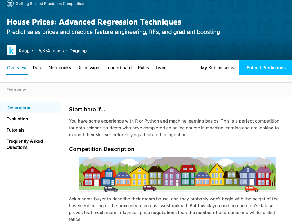
house-prices-advanced-regression-techniques 2030-01-01 00:00:00 Getting Started Knowledge 5364 True
connectx 2030-01-01 00:00:00 Getting Started Knowledge 389 False
nlp-getting-started 2030-01-01 00:00:00 Getting Started Kudos 1704 True
competitive-data-science-predict-future-sales 2020-12-31 23:59:00 Playground Kudos 7210 False
siim-isic-melanoma-classification 2020-08-17 23:59:00 Featured $30,000 637 False
global-wheat-detection 2020-08-04 23:59:00 Research $15,000 714 False
open-images-object-detection-rvc-2020 2020-07-31 16:00:00 Playground Knowledge 22 False
open-images-instance-segmentation-rvc-2020 2020-07-31 16:00:00 Playground Knowledge 5 False
hashcode-photo-slideshow 2020-07-27 23:59:00 Playground Knowledge 33 False
prostate-cancer-grade-assessment 2020-07-22 23:59:00 Featured $25,000 531 False
alaska2-image-steganalysis 2020-07-20 23:59:00 Research $25,000 471 False
halite 2020-06-30 23:59:00 Featured Kudos 0 False
m5-forecasting-accuracy 2020-06-30 23:59:00 Featured $50,000 4749 True
m5-forecasting-uncertainty 2020-06-30 23:59:00 Featured $50,000 572 False
trends-assessment-prediction 2020-06-29 23:59:00 Research $25,000 597 False
jigsaw-multilingual-toxic-comment-classification 2020-06-22 23:59:00 Featured $50,000 1277 False
tweet-sentiment-extraction 2020-06-16 23:59:00 Featured $15,000 1869 False
trec-covid-information-retrieval 2020-06-03 11:00:00 Research Kudos 19 False
- 여기에서 참여하기 원하는 대회의 데이터셋을 불러오면 된다.
- 이번
basic강의에서는house-prices-advanced-regression-techniques데이터를 활용한데이터 가공과 시각화를 연습할 것이기 때문에 아래와 같이 코드를 실행하여 데이터를 불러온다.
!kaggle competitions download -c house-prices-advanced-regression-techniques
Warning: Looks like you're using an outdated API Version, please consider updating (server 1.5.6 / client 1.5.4)
Downloading sample_submission.csv to /content/drive/My Drive/Colab Notebooks/inflearn_kaggle/data
  0% 0.00/31.2k [00:00<?, ?B/s]
100% 31.2k/31.2k [00:00<00:00, 4.73MB/s]
Downloading train.csv to /content/drive/My Drive/Colab Notebooks/inflearn_kaggle/data
  0% 0.00/450k [00:00<?, ?B/s]
100% 450k/450k [00:00<00:00, 30.0MB/s]
Downloading test.csv to /content/drive/My Drive/Colab Notebooks/inflearn_kaggle/data
  0% 0.00/441k [00:00<?, ?B/s]
100% 441k/441k [00:00<00:00, 29.0MB/s]
Downloading data_description.txt to /content/drive/My Drive/Colab Notebooks/inflearn_kaggle/data
  0% 0.00/13.1k [00:00<?, ?B/s]
100% 13.1k/13.1k [00:00<00:00, 1.83MB/s]
!ls
data_description.txt sample_submission.csv test.csv train.csv
- 현재 총 4개의 데이터를 다운로드 받았다.
- data_description.txt
- sample_submission.csv
- test.csv
- train.csv
VI. What’s Next
Google Colab에서Kaggle API를 활용하여 데이터를 불러오는 것을 실습하였다.Kaggle에서 받은 데이터를구글 드라이브에 바로 저장하는 방법을 배웠다.- 다음 시간에는 데이터를 불러온 뒤 이제 본격적인 EDA를 단계별로 진행한다. (Stay with Me)
VII. 옵션
- 구글 코랩은 참고로 한글폰트를 지원하지 않는다. 따라서, 한글 폰트를 꼭 실무에서 사용하고 싶은 분들은 아래
Reference에 관련 내용을 같이 첨부한 것이 있으니 확인하시기를 바란다. - 본 튜토리얼에서 Kaggle 데이터는 모두 영어이기에 한글폰트는 따로 사용하지 않는다.
Reference
EDA with Pandas - Data Merge
강의 홍보
- 취준생을 위한 강의를 제작하였습니다.
- 본 블로그를 통해서 강의를 수강하신 분은 게시글 제목과 링크를 수강하여 인프런 메시지를 통해 보내주시기를 바랍니다.
스타벅스 아이스 아메리카노를 선물로 보내드리겠습니다.
- [비전공자 대환영] 제로베이스도 쉽게 입문하는 파이썬 데이터 분석 - 캐글입문기

I. 개요
- 실무 데이터에서는 여러가지 데이터를 만나는 경우가 흔하다.
- 이 때,
SQL에서 데이터를 직접 병합하는 방법이 좋다. - 그러나, 현실적으로
DB에 접근하는 권한을 가진 경우는 흔하지는 않다. 현재 운영중인 서비스상에DB를 직접 만지는 경우는 거의 없다 (DBA가 할지도..) - 따라서, 데이터분석가는 흩어져 있는 데이터
Dump를 받게 될 가능성이 큰데, 이 때 Python에서 데이터를 병합하는 작업을 진행하게 된다. Kaggle이나 각종 경진대회에 출전하게 되면 서로 다른 데이터를 합쳐야 하는 경우가 매우 많다.
II. 모듈 Import
- 패키지 설치방법은 설치 문서를 확인한다.
import pandas as pd
print(pd.__version__)
1.0.4
- 데이터프레임을 보다 이쁘게 출력하기 위해 다음 2개의 패키지를 불러온다.
from IPython.core.display import display, HTML
from tabulate import tabulate
III. Pandas 데이터 병합 Sample Tutorial
- 간단하게 데이터를 병합하는 방법에 대해 실습을 진행한다.
- 데이터와 소스 코드는 Pandas 공식 홈페이지에서 한글 형태로 조금 수정했다.
(1) 파라미터 세팅
- 먼저, 행과 열을 최대 출력하는 개수를 지정한다.
pd.set_option('display.max_columns', 500)
pd.set_option('display.max_rows', 500)
(2) 데이터 생성
- 먼저 가상의 데이터를 두개 만든다.
temp_1 = pd.DataFrame({'key': ['A', 'B', 'C', 'D'],
                       'num1': [1,2,3,4]})
print(tabulate(temp_1, headers=['key', 'num'], tablefmt='pipe'))
|    | key   |   num |
|---:|:------|------:|
|  0 | A     |     1 |
|  1 | B     |     2 |
|  2 | C     |     3 |
|  3 | D     |     4 |
temp_2 = pd.DataFrame({'key': ['A', 'B', 'E', 'F'],
                       'num2': [5,6,7,8]})
print(tabulate(temp_2, headers=['key', 'num'], tablefmt='pipe'))
|    | key   |   num |
|---:|:------|------:|
|  0 | A     |     5 |
|  1 | B     |     6 |
|  2 | E     |     7 |
|  3 | F     |     8 |
(3) Data Merge - inner join
key값을 근거로 데이터를 병합한다.- 이 때, merge의 형태는
inner join형태로 출력된다.
merge_df = pd.merge(temp_1, temp_2, on='key')
print(tabulate(merge_df, headers=['key', 'num1', 'num2'], tablefmt='pipe'))
|    | key   |   num1 |   num2 |
|---:|:------|-------:|-------:|
|  0 | A     |      1 |      5 |
|  1 | B     |      2 |      6 |
inner_df = pd.merge(temp_1, temp_2, on='key', how='inner')
print(tabulate(inner_df, headers=['key', 'num1', 'num2'], tablefmt='pipe'))
|    | key   |   num1 |   num2 |
|---:|:------|-------:|-------:|
|  0 | A     |      1 |      5 |
|  1 | B     |      2 |      6 |
- 위 두개의 결과값이 똑같음을 확인할 수 있다.
(4) Data Merge - outer join
- 이번에는
outer join을 해보자.
outer_df = pd.merge(temp_1, temp_2, on='key', how='outer')
print(tabulate(outer_df, headers=['key', 'num1', 'num2'], tablefmt='pipe'))
|    | key   |   num1 |   num2 |
|---:|:------|-------:|-------:|
|  0 | A     |      1 |      5 |
|  1 | B     |      2 |      6 |
|  2 | C     |      3 |    nan |
|  3 | D     |      4 |    nan |
|  4 | E     |    nan |      7 |
|  5 | F     |    nan |      8 |
- 결과값을 보면, 우선
key값은 모두 출력되었다. - 이 때, 각 데이터에서 가져오는
num1과num2의Column도 같이 들어오는데, 각column마다 없는 값들은 이렇게nan으로 조회됨을 확인할 수 있다.
(5) Assignment
- 이제 수강생 분들이
left&right조인을 해보도록 한다. - 공식문서를 보면서 코드 작성하는 것을 추천한다.
- Merge, join, and concatenate
- 먼저
right join을 해본다.
# pd.merge(temp_1, temp_2) 여기 코드에서 남은 코드를 작성하면 됩니다.
right_df = pd.merge(temp_1, temp_2, on='key', how='left')
print(tabulate(right_df, headers=['key', 'num1', 'num2'], tablefmt='pipe'))
|    | key   |   num1 |   num2 |
|---:|:------|-------:|-------:|
|  0 | A     |      1 |      5 |
|  1 | B     |      2 |      6 |
|  2 | E     |    nan |      7 |
|  3 | F     |    nan |      8 |
- 그리고 이번에는
left join을 해본다.
# pd.merge(temp_1, temp_2) 여기 코드에서 남은 코드를 작성하면 됩니다.
right_df = pd.merge(temp_1, temp_2, on='key', how='left')
print(tabulate(right_df, headers=['key', 'num1', 'num2'], tablefmt='pipe'))
|    | key   |   num1 |   num2 |
|---:|:------|-------:|-------:|
|  0 | A     |      1 |      5 |
|  1 | B     |      2 |      6 |
|  2 | C     |      3 |    nan |
|  3 | D     |      4 |    nan |
VI. What’s next
- 데이터를 병합하는 방법 중
Merge에 대해서 배웠다. Merge에는 크게 4가지 방법이 있고, 방법에 따라서 최종 데이터의 출력값이 서로 다름을 확인하였다.- 다음 시간에는 또다른 병합 방법인
Concatenate에 학습하도록 한다.
EDA with Personal Email - Data Import
강의 홍보
- 취준생을 위한 강의를 제작하였습니다.
- 본 블로그를 통해서 강의를 수강하신 분은 게시글 제목과 링크를 수강하여 인프런 메시지를 통해 보내주시기를 바랍니다.
스타벅스 아이스 아메리카노를 선물로 보내드리겠습니다.
- [비전공자 대환영] 제로베이스도 쉽게 입문하는 파이썬 데이터 분석 - 캐글입문기
공지
제 수업을 듣는 사람들이 계속적으로 실습할 수 있도록 강의 파일을 만들었습니다. 늘 도움이 되기를 바라며. 참고했던 교재 및 Reference는 꼭 확인하셔서 교재 구매 또는 관련 Reference를 확인하시기를 바랍니다.
I. Matplotlib & Seaborn
(1) 기본 개요
Matplotlib는 파이썬 표준 시각화 도구라고 불리워지며 파이썬 그래프의 기본 토대가 된다고 해도 무방하다. 객체지향 프로그래밍을 지원하므로 세세하게 꾸밀 수 있다.
Chapter_1_2_Python_visualisation_seaborn
공지
제 수업을 듣는 사람들이 계속적으로 실습할 수 있도록 강의 파일을 만들었습니다. 늘 도움이 되기를 바라며. 참고했던 교재 및 Reference는 꼭 확인하셔서 교재 구매 또는 관련 Reference를 확인하시기를 바랍니다.
I. Matplotlib & Seaborn
(1) 기본 개요
Matplotlib는 파이썬 표준 시각화 도구라고 불리워지며 파이썬 그래프의 기본 토대가 된다고 해도 무방하다. 객체지향 프로그래밍을 지원하므로 세세하게 꾸밀 수 있다.
Seaborn 그래는 파이썬 시각화 도구의 고급 버전이다. Matplotlib에 비해 비교적 단순한 인터페이스를 제공하기 때문에 초보자도 어렵지 않게 배울 수 있다.
Chapter_1_1_Python_visualisation_intro

공지
제 수업을 듣는 사람들이 계속적으로 실습할 수 있도록 강의 파일을 만들었습니다. 늘 도움이 되기를 바라며. 참고했던 교재 및 Reference는 꼭 확인하셔서 교재 구매 또는 관련 Reference를 확인하시기를 바랍니다.
I. Matplotlib
(1) 기본 개요
Matplotlib는 파이썬 표준 시각화 도구라고 불리워지며 파이썬 그래프의 기본 토대가 된다고 해도 무방하다. 객체지향 프로그래밍을 지원하므로 세세하게 꾸밀 수 있다.
Seaborn 그래는 파이썬 시각화 도구의 고급 버전이다. Matplotlib에 비해 비교적 단순한 인터페이스를 제공하기 때문에 초보자도 어렵지 않게 배울 수 있다.
EDA with Python - Pandas
강의 홍보
- 취준생을 위한 강의를 제작하였습니다.
- 본 블로그를 통해서 강의를 수강하신 분은 게시글 제목과 링크를 수강하여 인프런 메시지를 통해 보내주시기를 바랍니다.
스타벅스 아이스 아메리카노를 선물로 보내드리겠습니다.
- [비전공자 대환영] 제로베이스도 쉽게 입문하는 파이썬 데이터 분석 - 캐글입문기
![]()
I. 개요
Pandas는panel data의 의미를 가지고 있다.- 흔히, 엑셀 데이터로 불리우는
관계형(Relational)또는레이블링된(Labeling)된 데이터를 보다 쉽게, 직관적으로 작업할 수 있도록 설계되어 있다. Python에서 데이터 분석을 수행하기 위한 매우 기초적이며 높은 수준의 문법을 제공한다.Pandas는 크게Series&DataFrame을 다룰 수 있도록 기초 문법을 제공하고 있다.Pandas가 다루는 여러 종류의 데이터를 확인해보자.- SQL 테이블 또는 Excel 스프레드시트에서와 같이 형식의 행과 열이 있는 표 형식 데이터
- 순서 및 순서 지정되지 않은(고정 빈도일 필요는 없음) 시계열 데이터.
- 행 및 열 레이블이 있는 임의 행렬 데이터(동일하게 입력 또는 이기종)
- 기타 형태의 관측/통계 데이터 세트
II. 모듈 Import
- 패키지 설치방법은 설치 문서를 확인한다.
import pandas as pd
print(pd.__version__)
1.0.3
III. Pandas 기본 활용법
Pandas가 제공하는 다양한 기능은 다음과 같지만, 본 튜토리얼에서는Sample위주로 다루도록 한다.- 부동 소수점 데이터뿐만 아니라 부동 소수점 데이터에서도 결측 데이터(NaN으로 표시됨)를 쉽게 처리함
- 크기 변이성: DataFrame 및 고차원 객체에서 열을 삽입 및 삭제 가능
- 자동 및 명시적 데이터 정렬: 객체를 라벨 집합에 명시적으로 정렬하거나, 사용자가 라벨을 무시하고
Series,DataFrame등이 자동으로 데이터를 계산에서 정렬 가능 - 데이터 집합에서 데이터 집합의 분할 적용 결합 작업을 수행할 수 있는 기능
- 다른
Python및NumPy데이터 구조에서 색인이 다른 데이터를DataFrame개체로 쉽게 변환 - 지능형 라벨 기반 슬라이싱, 고급 인덱싱 및 대용량 데이터 세트 부분 집합 취하기
- 직관적인 데이터 세트 병합 및 결합
- 유연한 데이터 세트 재구성 및 피벗테이블 구성
- 축의 계층적 라벨링(눈금당 여러 개의 라벨을 가질 수 있음)
- 플랫 파일(CSV 및 구분), Excel 파일, 데이터베이스 로딩 및 초고속 HDF5 형식의 데이터 저장/로딩에 사용되는 강력한 데이터 IO 도구
- 시계열별 기능: 날짜 범위 생성 및 주파수 변환, 이동 창 통계, 날짜 이동 및 지연.
IV. Pandas Sample Tutorial
- 간단하게
Pandas를 활용한Tutorial을 확인해보자.
(1) 파라미터 세팅
- 먼저, 행과 열을 최대 출력하는 개수를 지정한다.
pd.set_option('display.max_columns', 500)
pd.set_option('display.max_rows', 500)
(2) 데이터 생성
- 데이터를 생성하는 방법은 크게 2가지로 구분된다. (
Series,DataFrame)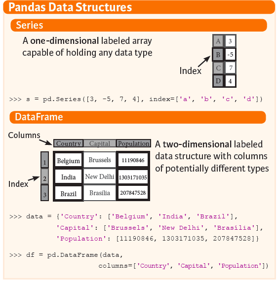
- 먼저
Series를 만들어보자.
temp_series = pd.Series([1,2,3,5,8,13,21])
print(temp_series)
0     1
1     2
2     3
3     5
4     8
5    13
6    21
dtype: int64
- 이제
Series에 있는 데이터와 함께DataFrame을 만든다.
series_df = pd.DataFrame({
    "No":range(1,5),
    "날짜":pd.Timestamp('20200601'),
    "출석점수":pd.Series(5, index=list(range(4)), dtype='float64'),
    "등급":pd.Categorical(["A등급", "B등급", "C등급", "D등급"]),
    "구분":"학점"
})

print(series_df)
   No         날짜  출석점수   등급  구분
0   1 2020-06-01   5.0  A등급  학점
1   2 2020-06-01   5.0  B등급  학점
2   3 2020-06-01   5.0  C등급  학점
3   4 2020-06-01   5.0  D등급  학점
- 이번에는 딕셔너리에서 데이터프레임으로 변환하는 소스코드다.
- 아래 코드에서 보여주고자 하는 것은 딕셔너리의 크기가 동일하지 않아도, 데이터프레임으로 변환되는데 문제가 없다.
- 다만,
NaN으로 채울 뿐이다.
dict_df = [{'가': '사과', '나': '볼'},{'가': '비행기', '나': '방망이', '다': '고양이'}]
dict_df = pd.DataFrame(dict_df)
print(dict_df)
     가    나    다
0   사과    볼  NaN
1  비행기  방망이  고양이
- 이번에는 배열에서 데이터프레임으로 변환하는 소스코드다.
sdf = {
    '국가':['한국', '미국', '일본'],
    'ISO-Code':[1,2,3],
    '지역': [4180.69, 4917.94, 454.07,],
    '위치': ["서울", "LA", "동경"]
    }
sdf = pd.DataFrame(sdf)
print(sdf)
   국가  ISO-Code       지역  위치
0  한국         1  4180.69  서울
1  미국         2  4917.94  LA
2  일본         3   454.07  동경
(3) 파일 입출력
- 외부 데이터의 파일 입출력에 대한 코드를 입력한다.
url = 'http://archive.ics.uci.edu/ml/machine-learning-databases/adult/adult.data'
df = pd.read_csv(url)
print(df.head(2))
   39          State-gov   77516   Bachelors   13        Never-married  \
0  50   Self-emp-not-inc   83311   Bachelors   13   Married-civ-spouse
1  38            Private  215646     HS-grad    9             Divorced

         Adm-clerical   Not-in-family   White   Male   2174   0   40  \
0     Exec-managerial         Husband   White   Male      0   0   13
1   Handlers-cleaners   Not-in-family   White   Male      0   0   40

    United-States   <=50K
0   United-States   <=50K
1   United-States   <=50K
- 컬럼명이 지정되지 않아 관측값이 컬럼명 위치에 있는 것을 확인할 수 있다.
- 이 때에는 컬럼명을 먼저 저장한 뒤, 아래와 같은 코드로 실행하면 정상적으로 데이터프레임이 완성된다.
columns = ['age', 'workclass', 'fnlwgt', 'education', 'education_num',
           'marital_status', 'occupation', 'relationship', 'ethnicity',
           'gender','capital_gain','capital_loss','hours_per_week','country_of_origin','income']

df2 = pd.read_csv(url, names=columns)
print(df2.head(2))
   age          workclass  fnlwgt   education  education_num  \
0   39          State-gov   77516   Bachelors             13
1   50   Self-emp-not-inc   83311   Bachelors             13

        marital_status        occupation    relationship ethnicity gender  \
0        Never-married      Adm-clerical   Not-in-family     White   Male
1   Married-civ-spouse   Exec-managerial         Husband     White   Male

   capital_gain  capital_loss  hours_per_week country_of_origin  income
0          2174             0              40     United-States   <=50K
1             0             0              13     United-States   <=50K
- 컬럼명에 대한 정보는 Adult Data Set 에서 참고한다.
- 판다스를 배울 때 조금더 자세히 배우겠지만,
info()함수를 사용하면 데이터의 일반적인 정보를 확인할 수 있다.
print(df2.info())
<class 'pandas.core.frame.DataFrame'>
RangeIndex: 32561 entries, 0 to 32560
Data columns (total 15 columns):
 #   Column             Non-Null Count  Dtype
---  ------             --------------  -----
 0   age                32561 non-null  int64
 1   workclass          32561 non-null  object
 2   fnlwgt             32561 non-null  int64
 3   education          32561 non-null  object
 4   education_num      32561 non-null  int64
 5   marital_status     32561 non-null  object
 6   occupation         32561 non-null  object
 7   relationship       32561 non-null  object
 8   ethnicity          32561 non-null  object
 9   gender             32561 non-null  object
 10  capital_gain       32561 non-null  int64
 11  capital_loss       32561 non-null  int64
 12  hours_per_week     32561 non-null  int64
 13  country_of_origin  32561 non-null  object
 14  income             32561 non-null  object
dtypes: int64(6), object(9)
memory usage: 3.7+ MB
None
V. 결론
- 간단하게
Pandas를 활용한 데이터 생성 및 파일 입출력에 대해서 배우는 시간을 가졌다. - 만약, 빠르게 판다스를 활용하여 데이터 전처리를 연습 하고 싶다면, 공식홈페이지에 있는 10 minutes to pandas에서 학습하는 것을 권장한다.
- 강사는
Kaggle데이터를 활용하여Pandas함수를 응용할 것이다.
Reference
Mukhiya, Suresh Kumar, and Usman Ahmed. “Hands-On Exploratory Data Analysis with Python.” Packt Publishing, Mar. 2020, www.packtpub.com/data/hands-on-exploratory-data-analysis-with-python.
EDA with Python - NumPy Broadcasting
강의 홍보
- 취준생을 위한 강의를 제작하였습니다.
- 본 블로그를 통해서 강의를 수강하신 분은 게시글 제목과 링크를 수강하여 인프런 메시지를 통해 보내주시기를 바랍니다.
스타벅스 아이스 아메리카노를 선물로 보내드리겠습니다.
- [비전공자 대환영] 제로베이스도 쉽게 입문하는 파이썬 데이터 분석 - 캐글입문기
공지
제 수업을 듣는 사람들이 계속적으로 실습할 수 있도록 강의 파일을 만들었습니다. 늘 도움이 되기를 바라며. 참고했던 교재 및 Reference는 꼭 확인하셔서 교재 구매 또는 관련 Reference를 확인하시기를 바랍니다.

I. 개요
NumPy는 C언어로 구성되었으며, 고성능의 수치계산을 위해 나온 패키지이며,Numerical Python의 약자이다.Python을 활용한 데이터 분석을 수행할 때, 그리고 데이터 시각화나 전처리를 수행할 때,NumPy는 매우 자주 사용되기 때문에 한번쯤은 꼭 다듬고 가는 것이 중요하다.- 이전 포스트에서는 Python - NumPy 소개 및 다양한 객체 생성에 대해 다루었으니, 본 포스트 읽기에 앞서서 기본적인 개념에 대해 확인하기를 바란다.
II. 모듈 Import
- 패키지 설치방법은 설치 문서를 확인한다.
import numpy as np
print(np.__version__)
1.18.4
III. NumPy 기본 활용법
- NumPy 객체 생성을 한 뒤에, 파일 저장, 서로 다른 배열끼리의 사칙연산 등을 수행할 수 있다.
(1) NumPy 객체 파일 저장 및 불러오기
savetxt,loadtxt, 그리고genfromtxt함수를 활용하여 객체를 불러오는 예제를 실습한다.
# 객체 생성 후 저장하기
x = np.arange(0.0, 50.0, 1.0)
print(x)
np.savetxt('data.out', x, delimiter=',')
[ 0.  1.  2.  3.  4.  5.  6.  7.  8.  9. 10. 11. 12. 13. 14. 15. 16. 17.
 18. 19. 20. 21. 22. 23. 24. 25. 26. 27. 28. 29. 30. 31. 32. 33. 34. 35.
 36. 37. 38. 39. 40. 41. 42. 43. 44. 45. 46. 47. 48. 49.]
!ls
data.out sample_data
- 현재 폴더에
data.out파일이 생성된 것을 확인할 수 있다.
# `data.out` 불러오기
z = np.loadtxt('data.out', unpack=True)
print(z)
[ 0.  1.  2.  3.  4.  5.  6.  7.  8.  9. 10. 11. 12. 13. 14. 15. 16. 17.
 18. 19. 20. 21. 22. 23. 24. 25. 26. 27. 28. 29. 30. 31. 32. 33. 34. 35.
 36. 37. 38. 39. 40. 41. 42. 43. 44. 45. 46. 47. 48. 49.]
- 정상적으로
data.out을 불러와서z객체에 저장된 것을 확인할 수 있다.
# genfromtxt 활용
my_array2 = np.genfromtxt('data.out',
                          skip_header=1,
                          filling_values=-999)
print(my_array2)
[ 1.  2.  3.  4.  5.  6.  7.  8.  9. 10. 11. 12. 13. 14. 15. 16. 17. 18.
 19. 20. 21. 22. 23. 24. 25. 26. 27. 28. 29. 30. 31. 32. 33. 34. 35. 36.
 37. 38. 39. 40. 41. 42. 43. 44. 45. 46. 47. 48. 49.]
z객체와 마찬가지로my_array2도 객체가 정상적으로 생성된 것을 확인할 수 있다.
EDA with Python - NumPy basic
강의 홍보
- 취준생을 위한 강의를 제작하였습니다.
- 본 블로그를 통해서 강의를 수강하신 분은 게시글 제목과 링크를 수강하여 인프런 메시지를 통해 보내주시기를 바랍니다.
스타벅스 아이스 아메리카노를 선물로 보내드리겠습니다.
- [비전공자 대환영] 제로베이스도 쉽게 입문하는 파이썬 데이터 분석 - 캐글입문기
공지
제 수업을 듣는 사람들이 계속적으로 실습할 수 있도록 강의 파일을 만들었습니다. 늘 도움이 되기를 바라며. 참고했던 교재 및 Reference는 꼭 확인하셔서 교재 구매 또는 관련 Reference를 확인하시기를 바랍니다.
I. 개요
- 파이썬 처음 입문하는 사람들을 위해서 작성하였다.
탐색작 자료분석(EDA: Exploratory Data Analysis)을 위해 가장 기초적인 뼈대가 되는NumPy에 대해서 학습하도록 합니다.
II. Array 만들기
- 1차원, 2차원, 3차원의 Array를 만들고 학습니다.
- 먼저
numpy라이브러리를 불러옵니다.
# import numpy
import numpy as np
print(np.__version__)
1.18.4
- 현재 구글 코랩에서 제공하는
numpy 버전은 1.18.4로 확인되고 있습니다.
(1) 1차원 Array 만들기
- 1차원 Array를 만들어 봅시다.
my_1D_array = np.array([1,3,5,7])
print(my_1D_array)
type(my_1D_array)
[1 3 5 7]


numpy.ndarray
(2) 2차원 Array 만들기
- 이번에는 2차원 Array를 만듭니다.
my_2D_array = np.array([[1, 2, 3, 4], [2, 4, 9, 16], [4, 8, 18, 32]])
print(my_2D_array)
type(my_2D_array)
[[ 1  2  3  4]
 [ 2  4  9 16]
 [ 4  8 18 32]]


numpy.ndarray
(3) 3차원 Array 만들기
- 이번에는 3차원 Array를 만듭니다.
my_3D_array = np.array([[[ 1, 2 , 3 , 4],[ 5 , 6 , 7 ,8]], [[ 1, 2, 3, 4],[ 9, 10, 11, 12]]])
print(my_3D_array)
type(my_3D_array)
[[[ 1  2  3  4]
  [ 5  6  7  8]]

 [[ 1  2  3  4]
  [ 9 10 11 12]]]


numpy.ndarray
III. Array Information
- 실무에서는 데이터를 어떤 형태로 수집되는지 바로 판단하기가 어렵습니다.
- 따라서, 수집받은 데이터를 다양한 방식으로 출력하여 정보를 알아가는 것이 좋습니다.
- 대표적으로, ndim, shape, dtype을 통해서 확인합니다.
- ndim은 배열의 차원수를 의미합니다.
- shape는 tuple의 index개수와 각 index가 보유하는 elements의 개수를 반환합니다.
- dtype는 각 게체의 데이터 타입을 표시합니다.
(1) 함수 작성
- 저장된 1차원, 2차원, 3차원의 Array를 활용합니다.
- 먼저, 빠르게 확인하기 위해 함수를 작성합니다.
def check_array_info(arr_obj):
  if isinstance(arr_obj, (np.ndarray)):
    print("The current dimension is :", arr_obj.ndim)
    print("The current shape is :", arr_obj.shape)
    print("The current dtype is :", arr_obj.dtype)
    print("The current value is :\n", arr_obj)
(1) 1차원 Array의 정보 확인
- 이제 정보를 확인합니다.
check_array_info(my_1D_array)
The current dimension is : 1
The current shape is : (4,)
The current dtype is : int64
The current value is :
 [1 3 5 7]
- 1차원 shape의 경우에는 (4,)만 표시가 되었는데, 이는 요소의 개수만 출력됨을 의미합니다.
(2) 2차원 Array의 정보 확인
- 2차원 배열의 정보를 확인합니다.
check_array_info(my_2D_array)
The current dimension is : 2
The current shape is : (3, 4)
The current dtype is : int64
The current value is :
 [[ 1  2  3  4]
 [ 2  4  9 16]
 [ 4  8 18 32]]
(3) 3차원 Array의 정보 확인
- 3차원 배열의 정보를 확인합니다.
check_array_info(my_3D_array)
The current dimension is : 3
The current shape is : (2, 2, 4)
The current dtype is : int64
The current value is :
 [[[ 1  2  3  4]
  [ 5  6  7  8]]

 [[ 1  2  3  4]
  [ 9 10 11 12]]]
IV. Creating An Array
- 이제 다양한 방식으로 NumPy를 작성해보자.
# Array of ones
ones = np.ones((3,4))
check_array_info(ones)
The current dimension is : 2
The current shape is : (3, 4)
The current dtype is : float64
The current value is :
 [[1. 1. 1. 1.]
 [1. 1. 1. 1.]
 [1. 1. 1. 1.]]
# Array of zeros
zeros = np.zeros((1,2,3), dtype=np.int16)
check_array_info(zeros)
The current dimension is : 3
The current shape is : (1, 2, 3)
The current dtype is : int16
The current value is :
 [[[0 0 0]
  [0 0 0]]]
# Array with random values
np_random = np.random.random((2,2))
check_array_info(np_random)
The current dimension is : 2
The current shape is : (2, 2)
The current dtype is : float64
The current value is :
 [[0.47775118 0.60277821]
 [0.01818544 0.23499141]]
# Empty Array
empty_array = np.empty((3,2))
check_array_info(empty_array)
The current dimension is : 2
The current shape is : (3, 2)
The current dtype is : float64
The current value is :
 [[2.31101775e-316 0.00000000e+000]
 [0.00000000e+000 0.00000000e+000]
 [0.00000000e+000 0.00000000e+000]]
# Full Array
full_array = np.full((2,2), 7)
check_array_info(full_array)
The current dimension is : 2
The current shape is : (2, 2)
The current dtype is : int64
The current value is :
 [[7 7]
 [7 7]]
# Array of evenly_spaced values
even_spaced_array = np.arange(10, 25, 5)
check_array_info(even_spaced_array)
The current dimension is : 1
The current shape is : (3,)
The current dtype is : int64
The current value is :
 [10 15 20]
even_spaced_array2 = np.linspace(0, 2, 9)
check_array_info(even_spaced_array2)
The current dimension is : 1
The current shape is : (9,)
The current dtype is : float64
The current value is :
 [0.   0.25 0.5  0.75 1.   1.25 1.5  1.75 2.  ]
V. Array의 메모리 체크
- 머신러닝과 딥러닝을 수행하려면 반드시 메모리 체크가 필수다.
- 이 부분과 관련된 함수를 작성하여 기존에 저장된 1차원, 2차원, 3차원 배열의 객체를 출력하여 본다.
(1) 함수 작성
check_memory_info라는 함수를 만들어보자.
def check_memory_info(arr_obj):
  if isinstance(arr_obj, (np.ndarray)):
    print("The current size is :", arr_obj.size)
    print("The current flags is :", arr_obj.flags)
    print("The current itemzise is :", arr_obj.itemsize)
    print("The current total consumed bytes is :", arr_obj.nbytes)
size는element의 전체 개수를 의미한다.flags는memory layout의 정보를 출력한다.itemsize는 bytes 당 한 배열의 길이를 출력한다.nbytes는 객체가 소비하는 전체 bytes를 출력한다.
(1) 1차원 Array의 메모리 정보 확인
check_memory_info(my_1D_array)
The current size is : 4
The current flags is :   C_CONTIGUOUS : True
  F_CONTIGUOUS : True
  OWNDATA : True
  WRITEABLE : True
  ALIGNED : True
  WRITEBACKIFCOPY : False
  UPDATEIFCOPY : False

The current itemzise is : 8
The current total consumed bytes is : 32
(1) 2차원 Array의 메모리 정보 확인
check_memory_info(my_2D_array)
The current size is : 12
The current flags is :   C_CONTIGUOUS : True
  F_CONTIGUOUS : False
  OWNDATA : True
  WRITEABLE : True
  ALIGNED : True
  WRITEBACKIFCOPY : False
  UPDATEIFCOPY : False

The current itemzise is : 8
The current total consumed bytes is : 96
(3) 1차원 Array의 메모리 정보 확인
check_memory_info(my_3D_array)
The current size is : 16
The current flags is :   C_CONTIGUOUS : True
  F_CONTIGUOUS : False
  OWNDATA : True
  WRITEABLE : True
  ALIGNED : True
  WRITEBACKIFCOPY : False
  UPDATEIFCOPY : False

The current itemzise is : 8
The current total consumed bytes is : 128
VI. 결론
NumPy는 파이썬에서 다루는 데이터과학에서 다루는 매우 중요한 토대가 되는 라이브러이이다.- 간단하게
NumPy를 활용한 배열에 대해 학습하였다. - 또한,
Array를 다양하게 만들어보고,Array가 가지고 있는 다양한 정보를 확인할 수 있는 여러 함수에 대해 익히는 시간을 가졌다. - 그러나, 여기까지는 사실상 기초이고, 이제 배열의 연산에 대해 익히는 시간을 가져야 한다.
- 다음 시간에
Broadcasting이라는 기법을 학습할 것이다.
Reference
Mukhiya, Suresh Kumar, and Usman Ahmed. “Hands-On Exploratory Data Analysis with Python.” Packt Publishing, Mar. 2020, www.packtpub.com/data/hands-on-exploratory-data-analysis-with-python.