Data Visualisation

Convert Plotly Jupyterlab to HTML

개요

  • jupyter notebook에서 plotly 기반의 시각화를 작성한다.
  • jupyter notebook에서 html로 변환 시, plotly로 작성된 코드는 나타나지 않았다.
  • 이 때 필수적으로 입력해야 할 코드를 작성한다.

필수 코드 적용 전 변환 시

  • 간단한 시각화 코드를 작성 후, html로 변환한다.
import plotly.express as px

fig = px.line(x=["a","b","c"], y=[1,3,2], title="sample figure")
fig.show()
  • 아래 그림은 일반적으로 JupyterLab 에디터에서 HTML로 변환하는 과정이다.
    • File - Save and Export Notebook As… - HTML 순차적으로 클릭한다.

Screen Shot 2022-04-11 at 10.56.22 PM.png

Plot Tree 색상 변경

개요

  • skleran.tree.plot_tree의 색상을 바꿔보도록 한다.
  • matplotlib 객체지향의 구조를 알면 어렵지(?) 않게 바꿀 수 있다.
  • 간단하게 plot_tree 시각화를 구현해본다.
    • 언제나 예제로 희생당하는 iris 데이터에게 애도를 표한다.
  • 구글코랩에서 실행 시, 다음 코드를 실행하여 최신 라이브러리로 업그레이드 한다.
!pip install -U matplotlib
Requirement already satisfied: matplotlib in /usr/local/lib/python3.7/dist-packages (3.2.2)
Collecting matplotlib
  Downloading matplotlib-3.5.1-cp37-cp37m-manylinux_2_5_x86_64.manylinux1_x86_64.whl (11.2 MB)
     |████████████████████████████████| 11.2 MB 27.0 MB/s 
[?25hRequirement already satisfied: kiwisolver>=1.0.1 in /usr/local/lib/python3.7/dist-packages (from matplotlib) (1.4.0)
Requirement already satisfied: python-dateutil>=2.7 in /usr/local/lib/python3.7/dist-packages (from matplotlib) (2.8.2)
Requirement already satisfied: numpy>=1.17 in /usr/local/lib/python3.7/dist-packages (from matplotlib) (1.21.5)
Requirement already satisfied: pillow>=6.2.0 in /usr/local/lib/python3.7/dist-packages (from matplotlib) (7.1.2)
Requirement already satisfied: pyparsing>=2.2.1 in /usr/local/lib/python3.7/dist-packages (from matplotlib) (3.0.7)
Requirement already satisfied: cycler>=0.10 in /usr/local/lib/python3.7/dist-packages (from matplotlib) (0.11.0)
Requirement already satisfied: packaging>=20.0 in /usr/local/lib/python3.7/dist-packages (from matplotlib) (21.3)
Collecting fonttools>=4.22.0
  Downloading fonttools-4.31.2-py3-none-any.whl (899 kB)
     |████████████████████████████████| 899 kB 50.5 MB/s 
[?25hRequirement already satisfied: typing-extensions in /usr/local/lib/python3.7/dist-packages (from kiwisolver>=1.0.1->matplotlib) (3.10.0.2)
Requirement already satisfied: six>=1.5 in /usr/local/lib/python3.7/dist-packages (from python-dateutil>=2.7->matplotlib) (1.15.0)
Installing collected packages: fonttools, matplotlib
  Attempting uninstall: matplotlib
    Found existing installation: matplotlib 3.2.2
    Uninstalling matplotlib-3.2.2:
      Successfully uninstalled matplotlib-3.2.2
ERROR: pip's dependency resolver does not currently take into account all the packages that are installed. This behaviour is the source of the following dependency conflicts.
albumentations 0.1.12 requires imgaug<0.2.7,>=0.2.5, but you have imgaug 0.2.9 which is incompatible.
Successfully installed fonttools-4.31.2 matplotlib-3.5.1
%matplotlib inline 

import sklearn
print(sklearn.__version__)
import matplotlib
print(matplotlib.__version__)

# 필수 라이브러리 불러오기
from sklearn.datasets import load_iris
from sklearn import tree 
import matplotlib.pyplot as plt

# 데이터 불러오기
iris = load_iris()
print(iris.data.shape, iris.target.shape)
print("feature names", iris.feature_names)
print("class names", iris.target_names)

# 모형 학습 및 plot_tree 그래프 구현
dt = tree.DecisionTreeClassifier(random_state=0)
dt.fit(iris.data, iris.target)

fig, ax = plt.subplots(figsize=(10, 6))
ax = tree.plot_tree(dt, max_depth = 2, filled=True, feature_names = iris.feature_names, class_names = iris.target_names)
plt.show()
1.0.2
3.5.1
(150, 4) (150,)
feature names ['sepal length (cm)', 'sepal width (cm)', 'petal length (cm)', 'petal width (cm)']
class names ['setosa' 'versicolor' 'virginica']

png

Matplotlib 한글 폰트 추가 (Mac)

개요

  • Mac 유저를 위해 한글 폰트 추가하는 방법을 설명한다.
  • 기본 코드는 Windows에서도 동작한다.
  • 폰트 추가 방법은 생략한다.

한글 폰트 깨진 시각화

  • 간단하게 깨진 한글이 들어간 시각화를 구현한다.
import matplotlib.font_manager as fm
import matplotlib.pyplot as plt
import matplotlib as mpl
 
plt.plot([1, 2, 3, 4, 5])
plt.title("테스트")
plt.show()
/Library/Frameworks/Python.framework/Versions/3.8/lib/python3.8/site-packages/matplotlib/backends/backend_agg.py:238: RuntimeWarning: Glyph 53580 missing from current font.
  font.set_text(s, 0.0, flags=flags)
/Library/Frameworks/Python.framework/Versions/3.8/lib/python3.8/site-packages/matplotlib/backends/backend_agg.py:238: RuntimeWarning: Glyph 49828 missing from current font.
  font.set_text(s, 0.0, flags=flags)
/Library/Frameworks/Python.framework/Versions/3.8/lib/python3.8/site-packages/matplotlib/backends/backend_agg.py:238: RuntimeWarning: Glyph 53944 missing from current font.
  font.set_text(s, 0.0, flags=flags)
/Library/Frameworks/Python.framework/Versions/3.8/lib/python3.8/site-packages/matplotlib/backends/backend_agg.py:201: RuntimeWarning: Glyph 53580 missing from current font.
  font.set_text(s, 0, flags=flags)
/Library/Frameworks/Python.framework/Versions/3.8/lib/python3.8/site-packages/matplotlib/backends/backend_agg.py:201: RuntimeWarning: Glyph 49828 missing from current font.
  font.set_text(s, 0, flags=flags)
/Library/Frameworks/Python.framework/Versions/3.8/lib/python3.8/site-packages/matplotlib/backends/backend_agg.py:201: RuntimeWarning: Glyph 53944 missing from current font.
  font.set_text(s, 0, flags=flags)

png

Home Credit Default - Data Visualization

공지

  • 본 포스트는 재직자 교육을 위해 만든 강의안의 일부입니다.

Introduction

대회 개요

Many people struggle to get loans due to insufficient or non-existent credit histories. And, unfortunately, this population is often taken advantage of by untrustworthy lenders. Home Credit strives to broaden financial inclusion for the unbanked population by providing a positive and safe borrowing experience. In order to make sure this underserved population has a positive loan experience, Home Credit makes use of a variety of alternative data–including telco and transactional information–to predict their clients’ repayment abilities. While Home Credit is currently using various statistical and machine learning methods to make these predictions, they’re challenging Kagglers to help them unlock the full potential of their data. Doing so will ensure that clients capable of repayment are not rejected and that loans are given with a principal, maturity, and repayment calendar that will empower their clients to be successful.

matplotlib 03_2 Scatter Plot

강의 홍보

산점도 그래프

산점도는 두 수치형 변수의 분포를 비교하고 두 변수 사이에 상관 관계가 있는지 여부를 확인하는 데 사용됩니다. 데이터 내에 구별되는 군집/분할이 있으면 산점도에서도 명확해집니다.

(1) 라이브러리 불러오기

필요한 라이브러리를 불러옵니다.

import matplotlib.pyplot as plt
import numpy as np
import seaborn as sns

(2) 데이터 생성

이번에는 seaborn 패키지 내 tips 데이터를 활용합니다.

KDX Competition Guideline

개요

  • 본 수업을 듣는 수강생들을 위해 간단한 튜토리얼을 만들었다.
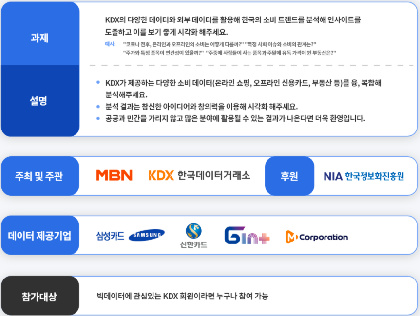
  • 대회는 다음과 같다.

/img/programming/2020/10/blog_kdx_guideline/img

1단계 패키지 불러오기

  • 데이터 가공 및 시각화 위주의 패키지를 불러온다.
library(tidyverse) # 데이터 가공 및 시각화
library(readxl) # 엑셀파일 불러오기 패키지 

2단계 데이터 불러오기

  • 데이터가 많아서 순차적으로 진행하도록 한다.
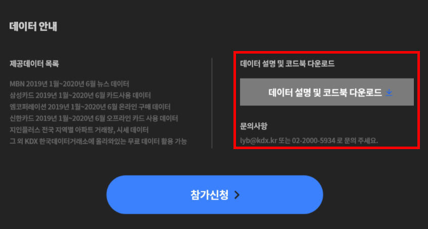
  • 각 데이터에 대한 설명은활용데이터설명(PDF)을 참조한다.

  • 먼저 제 개발환경은 아래와 같다.
    • Note: 윈도우와 Mac은 다를 수 있음을 명심하자.
sessionInfo()
## R version 4.0.2 (2020-06-22)
## Platform: x86_64-apple-darwin17.0 (64-bit)
## Running under: macOS Catalina 10.15.6
## 
## Matrix products: default
## BLAS:   /Library/Frameworks/R.framework/Versions/4.0/Resources/lib/libRblas.dylib
## LAPACK: /Library/Frameworks/R.framework/Versions/4.0/Resources/lib/libRlapack.dylib
## 
## locale:
## [1] en_US.UTF-8/en_US.UTF-8/en_US.UTF-8/C/en_US.UTF-8/en_US.UTF-8
## 
## attached base packages:
## [1] stats     graphics  grDevices utils     datasets  methods   base     
## 
## other attached packages:
##  [1] readxl_1.3.1    forcats_0.5.0   stringr_1.4.0   dplyr_1.0.0    
##  [5] purrr_0.3.4     readr_1.3.1     tidyr_1.1.0     tibble_3.0.3   
##  [9] ggplot2_3.3.2   tidyverse_1.3.0
## 
## loaded via a namespace (and not attached):
##  [1] Rcpp_1.0.5       cellranger_1.1.0 pillar_1.4.6     compiler_4.0.2  
##  [5] dbplyr_1.4.4     tools_4.0.2      digest_0.6.25    lubridate_1.7.9 
##  [9] jsonlite_1.7.0   evaluate_0.14    lifecycle_0.2.0  gtable_0.3.0    
## [13] pkgconfig_2.0.3  rlang_0.4.7      reprex_0.3.0     cli_2.0.2       
## [17] rstudioapi_0.11  DBI_1.1.0        yaml_2.2.1       haven_2.3.1     
## [21] xfun_0.16        withr_2.3.0      xml2_1.3.2       httr_1.4.2      
## [25] knitr_1.29       fs_1.5.0         hms_0.5.3        generics_0.0.2  
## [29] vctrs_0.3.2      grid_4.0.2       tidyselect_1.1.0 glue_1.4.1      
## [33] R6_2.4.1         fansi_0.4.1      rmarkdown_2.3    modelr_0.1.8    
## [37] blob_1.2.1       magrittr_1.5     backports_1.1.8  scales_1.1.1    
## [41] ellipsis_0.3.1   htmltools_0.5.0  rvest_0.3.6      assertthat_0.2.1
## [45] colorspace_1.4-1 stringi_1.4.6    munsell_0.5.0    broom_0.7.0     
## [49] crayon_1.3.4

(1) 삼성카드 데이터

  • 우선 삼성카드 데이터를 불러와서 확인한다.
  • 한글 파일은 인코딩이 늘 항상 문제다.
    • 파일을 불러오기 전 항상 파일 인코딩을 확인하도록 한다.
readr::guess_encoding("data/Samsungcard.csv", n_max = 100)
## # A tibble: 2 x 2
##   encoding confidence
##   <chr>         <dbl>
## 1 EUC-KR         1   
## 2 GB18030        0.62
  • Encoding 확인 결과 EUC-KR로 확인하였다.
samsung_card <- read_xlsx("data/Samsungcard.xlsx")
samsung_card2 <- read.csv("data/Samsungcard.csv", fileEncoding = "EUC-KR")
  • 위 두 파일이 동일한 것을 확인해본다
head(samsung_card)
## # A tibble: 6 x 5
##   소비일자 소비업종  성별  연령대 소비건수
##      <dbl> <chr>     <chr> <chr>     <dbl>
## 1 20190101 가전/가구 남성  20대       5529
## 2 20190101 가전/가구 남성  30대      17536
## 3 20190101 가전/가구 남성  40대      22838
## 4 20190101 가전/가구 남성  50대      15801
## 5 20190101 가전/가구 남성  60대       6772
## 6 20190101 가전/가구 여성  20대       5937
head(samsung_card2)
##   소비일자  소비업종 성별 연령대 소비건수
## 1 20190101 가전/가구 남성   20대     5529
## 2 20190101 가전/가구 남성   30대    17536
## 3 20190101 가전/가구 남성   40대    22838
## 4 20190101 가전/가구 남성   50대    15801
## 5 20190101 가전/가구 남성   60대     6772
## 6 20190101 가전/가구 여성   20대     5937
  • 두 파일이 동일한 것을 확인하였다면 이제 samsung_card2는 삭제를 한다.
    • RAM을 아껴 쓰자.
rm(samsung_card2) # 객체 지우는 함수
ls() # 현재 저장된 객체 확인하는 함수
## [1] "samsung_card"

(2) 신한카드 데이터

  • 이번에는 ShinhanCard.xslx 데이터를 불러온다.
shinhancard <- read_xlsx("data/Shinhancard.xlsx")
head(shinhancard)
## # A tibble: 6 x 8
##   일별    성별  연령대별 업종               `카드이용건수(천건)`… ...6  ...7   ...8
##   <chr>   <chr> <chr>    <chr>                           <dbl> <lgl> <lgl> <dbl>
## 1 201901… F     20대     M001_한식                       299.  NA    NA       10
## 2 201901… F     20대     M002_일식/중식/양식…               88.3 NA    NA       NA
## 3 201901… F     20대     M003_제과/커피/패스트푸드…              291.  NA    NA       NA
## 4 201901… F     20대     M004_기타요식                   446.  NA    NA       NA
## 5 201901… F     20대     M005_유흥                        24.2 NA    NA       NA
## 6 201901… F     20대     M006_백화점                      35.3 NA    NA       NA
  • 위 데이터를 불러오니 불필요한 6:8 변수가 불러온 것을 확인할 수 있다.
    • 실제 엑셀 데이터를 열어도 빈값임을 확인할 수 있다.
    • 따라서, 6:8 변수는 삭제한다.
shinhancard <- shinhancard %>% 
  select(-c(6:8))

head(shinhancard)
## # A tibble: 6 x 5
##   일별     성별  연령대별 업종                      `카드이용건수(천건)`
##   <chr>    <chr> <chr>    <chr>                                    <dbl>
## 1 20190101 F     20대     M001_한식                                299. 
## 2 20190101 F     20대     M002_일식/중식/양식                       88.3
## 3 20190101 F     20대     M003_제과/커피/패스트푸드                291. 
## 4 20190101 F     20대     M004_기타요식                            446. 
## 5 20190101 F     20대     M005_유흥                                 24.2
## 6 20190101 F     20대     M006_백화점                               35.3

(3) 지인플러스

  • 지인플러스는 아파트시세(GIN00009A)와 아파트 거래량(GIN00008B)을 담은 코드이다.
gin_8a <- read_csv("data/GIN00008A.csv")
gin_9a <- read_csv("data/GIN00009A.csv")
  • 위 두개의 데이터를 확인해본다.
glimpse(gin_8a)
## Rows: 937,904
## Columns: 9
## $ ym             <dbl> 200601, 200602, 200603, 200604, 200605, 200606, 200607…
## $ area_lvl_scor  <dbl> 0, 0, 0, 0, 0, 0, 0, 0, 0, 0, 0, 0, 0, 0, 0, 0, 0, 0, …
## $ lgdng_cd       <chr> "0000000000", "0000000000", "0000000000", "0000000000"…
## $ trd_cont       <dbl> 23357, 38617, 52241, 44253, 41916, 30257, 28613, 37362…
## $ avg_trd_cont   <dbl> 0, 0, 0, 0, 0, 0, 0, 0, 0, 0, 0, 0, 0, 0, 0, 0, 0, 0, …
## $ trd_deal_rat   <dbl> NA, NA, NA, NA, NA, NA, NA, NA, NA, NA, NA, NA, NA, NA…
## $ mtrnt_cont     <dbl> 0, 0, 0, 0, 0, 0, 0, 0, 0, 0, 0, 0, 0, 0, 0, 0, 0, 0, …
## $ avg_mtrnt_cont <dbl> 0, 0, 0, 0, 0, 0, 0, 0, 0, 0, 0, 0, 0, 0, 0, 0, 0, 0, …
## $ mtrnt_deal_rat <dbl> NA, NA, NA, NA, NA, NA, NA, NA, NA, NA, NA, NA, NA, NA…
glimpse(gin_9a)
## Rows: 785,805
## Columns: 4
## $ lgdng_cd <dbl> 1.1e+09, 1.1e+09, 1.1e+09, 1.1e+09, 1.1e+09, 1.1e+09, 1.1e+0…
## $ std_date <date> 2006-01-21, 2006-02-21, 2006-03-21, 2006-04-21, 2006-05-21,…
## $ trd_prc  <dbl> 1289, 1271, 1291, 1307, 1321, 1335, 1357, 1381, 1411, 1444, …
## $ ldpb_prc <dbl> NA, NA, NA, NA, NA, NA, NA, NA, NA, NA, NA, NA, NA, NA, NA, …

(4) JSON 파일 불러오기

  • JSON 파일 불러올 때에는 jsonlite 패키지를 활용한다.
library(jsonlite)
GIN_10m <- fromJSON("data/center_GIN00010M.json")
glimpse(GIN_10m)
## Rows: 20,572
## Columns: 8
## $ AREA_LVL_SCOR <int> 1, 2, 3, 3, 3, 3, 3, 3, 3, 3, 3, 3, 3, 3, 3, 3, 3, 3, 3…
## $ LGDNG_CD      <chr> "1100000000", "1111000000", "1111010100", "1111010200",…
## $ CTPV_NM       <chr> "서울특별시", "서울특별시", "서울특별시", "서울특별시", "서울특별시", "서울특별시", "…
## $ CTGG_NM       <chr> NA, "종로구", "종로구", "종로구", "종로구", "종로구", "종로구", "종로구", "종…
## $ EMD_NM        <chr> NA, NA, "청운동", "신교동", "궁정동", "효자동", "창성동", "통의동", "적선동"…
## $ LA            <dbl> 37.52934, 37.58586, 37.58920, 37.58449, 37.58468, 37.58…
## $ LNGT          <dbl> 126.9515, 126.9775, 126.9693, 126.9679, 126.9731, 126.9…
## $ PYN_CN        <chr> "{\"type\": \"Polygon\", \"coordinates\": [[[126.979658…
  • PYN_CN의 값이 조금 다른 것을 확인할 수 있다.
    • 이 부분은 추후 전처리할 때 정리하는 것으로 확인한다.

(5) SSC_Data

  • 이번에는 Mcorporation내 폴더 데이터를 올리도록 한다.
  • 이번에 파일을 불러올 때는 readr::read_csv()를 활용하여 불러온다.
readr::guess_encoding("data/Mcorporation/KDX시각화경진대회_SSC_DATA.csv")
## # A tibble: 2 x 2
##   encoding confidence
##   <chr>         <dbl>
## 1 EUC-KR         1   
## 2 GB18030        0.76
ssc_data <- read_csv("data/Mcorporation/KDX시각화경진대회_SSC_DATA.csv", locale = locale("ko", encoding = "EUC-KR"))
glimpse(ssc_data)
## Rows: 76,580
## Columns: 5
## $ 소비일자 <dbl> 20190101, 20190101, 20190101, 20190101, 20190101, 20190101, 2019…
## $ 소비업종 <chr> "가전/가구", "가전/가구", "가전/가구", "가전/가구", "가전/가구", "가전/가구", "가전/가구", "…
## $ 성별     <chr> "남성", "남성", "남성", "남성", "남성", "여성", "여성", "여성", "여성", "여성", "남…
## $ 연령대   <chr> "20대", "30대", "40대", "50대", "60대", "20대", "30대", "40대", "50대", …
## $ 소비건수 <dbl> 5529, 17536, 22838, 15801, 6772, 5937, 12895, 16896, 14025, 5909…

(6) 다중 엑셀파일 불러오기 예제

  • 상품 카데고리 데이터_KDX 시각화 폴더 내 엑셀 데이터를 확인해본다.
list.files(path = "data/Mcorporation/상품 카테고리 데이터_KDX 시각화 경진대회 Only/")
##  [1] "PC사무기기.xlsx"             "TV홈시어터.xlsx"            
##  [3] "가공식품.xlsx"               "가방지갑잡화.xlsx"          
##  [5] "건강관련용품.xlsx"           "건강식품.xlsx"              
##  [7] "계절가전.xlsx"               "골프용품.xlsx"              
##  [9] "공구류.xlsx"                 "구기.xlsx"                  
## [11] "국내외여행.xlsx"             "기타 스포츠.xlsx"           
## [13] "낚시.xlsx"                   "남성의류.xlsx"              
## [15] "노트북.xlsx"                 "농축수산물.xlsx"            
## [17] "도서음반DVD.xlsx"            "등산용품.xlsx"              
## [19] "메이크업.xlsx"               "문구사무용품.xlsx"          
## [21] "미용가전.xlsx"               "반려동물.xlsx"              
## [23] "생활가구.xlsx"               "생활가전.xlsx"              
## [25] "생활용품.xlsx"               "서비스티켓.xlsx"            
## [27] "성인용품.xlsx"               "세탁청소세면.xlsx"          
## [29] "수납가구.xlsx"               "수납용품.xlsx"              
## [31] "수영.xlsx"                   "스키보드.xlsx"              
## [33] "스킨케어.xlsx"               "스포츠의류.xlsx"            
## [35] "신발.xlsx"                   "악세서리시계주얼리.xlsx"    
## [37] "안전용품.xlsx"               "언더웨어.xlsx"              
## [39] "업소위생용품.xlsx"           "여성의류.xlsx"              
## [41] "완구키덜트게임.xlsx"         "욕실가전.xlsx"              
## [43] "욕실용품.xlsx"               "유아용품.xlsx"              
## [45] "유아패션.xlsx"               "음료.xlsx"                  
## [47] "음향가전.xlsx"               "인테리어용품.xlsx"          
## [49] "자동차용품.xlsx"             "자전거사이클보드인라인.xlsx"
## [51] "주방가전.xlsx"               "주방수납잡화.xlsx"          
## [53] "주방식기용기.xlsx"           "주방조리기구.xlsx"          
## [55] "출산임부용품.xlsx"           "취미악기.xlsx"              
## [57] "침실가구.xlsx"               "침실인테리어.xlsx"          
## [59] "카메라캠코더.xlsx"           "캠핑용품.xlsx"              
## [61] "테마의류.xlsx"               "헤어바디용품.xlsx"          
## [63] "헬스기구용품.xlsx"           "휴대폰악세서리.xlsx"
  • 몇가지 파일을 열어본다.
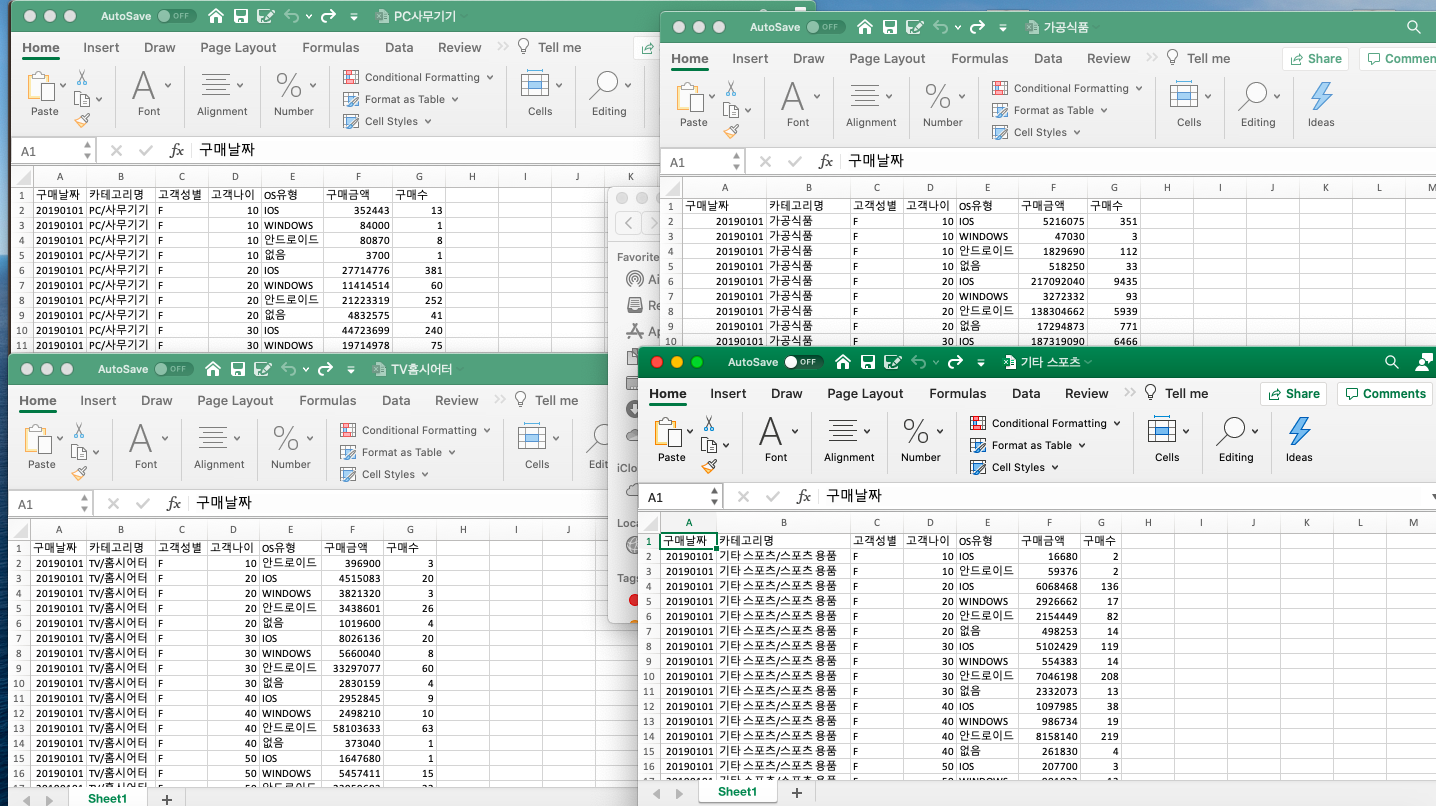
  • 엑셀 데이터의 변수 등이 동일한 것을 확인할 수 있다.
  • 이제 위 데이터를 한꺼번에 불러와서 하나의 데이터셋으로 합친다.
  • 검색키워드 Multiple Excel Files import in R
files <- list.files(path = "data/Mcorporation/상품 카테고리 데이터_KDX 시각화 경진대회 Only/", pattern = "*.xlsx", full.names = T)

products <- sapply(files, read_excel, simplify=FALSE) %>% 
  bind_rows(.id = "id") %>% 
  select(-id)

glimpse(products)
## Rows: 1,837,833
## Columns: 7
## $ 구매날짜   <dbl> 20190101, 20190101, 20190101, 20190101, 20190101, 20190101, 20…
## $ 카테고리명 <chr> "PC/사무기기", "PC/사무기기", "PC/사무기기", "PC/사무기기", "PC/사무기기", "PC/사무기기…
## $ 고객성별   <chr> "F", "F", "F", "F", "F", "F", "F", "F", "F", "F", "F", "F", "F…
## $ 고객나이   <dbl> 10, 10, 10, 10, 20, 20, 20, 20, 30, 30, 30, 30, 40, 40, 40, 40…
## $ OS유형     <chr> "IOS", "WINDOWS", "안드로이드", "없음", "IOS", "WINDOWS", "안드로이드", …
## $ 구매금액   <dbl> 352443, 84000, 80870, 3700, 27714776, 11414514, 21223319, 4832…
## $ 구매수     <dbl> 13, 1, 8, 1, 381, 60, 252, 41, 240, 75, 423, 19, 58, 110, 436…

3단계 데이터 시각화

  • 먼저, 데이터 저장 용량을 고려하여 products 데이터셋을 제외하고 나머지는 모두 삭제한다.
  • 데이터 시각화는 변수의 종류에 따른 시각화를 구현한 것이다.
  • 시각화 참조자료는 다음에서 작성이 가능하다.
  • 아래 샘플은 필자가 공부하는 형태를 구현한 것이다. 참조하기를 바란다.
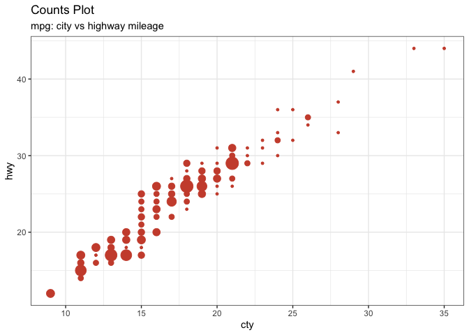
(1) 수치형 변수 ~ 수치형 변수

  • 수치형 변수 ~ 수치형 변수 시각화의 대표적인 기법은 산점도(scatter) 또는 correlation이라 부른다.
    • scatter 시각화를 구현한다.
# load package and data
library(ggplot2)
data(mpg, package="ggplot2")
# mpg <- read.csv("http://goo.gl/uEeRGu")

# Scatterplot
theme_set(theme_bw())  # pre-set the bw theme.
g <- ggplot(mpg, aes(cty, hwy))
g + geom_count(col="tomato3", show.legend=F) +
  labs(subtitle="mpg: city vs highway mileage", 
       y="hwy", 
       x="cty", 
       title="Counts Plot")

Seaborn Visualisation Tutorial - Basic

공지

제 수업을 듣는 사람들이 계속적으로 실습할 수 있도록 강의 파일을 만들었습니다. 늘 도움이 되기를 바라며. 참고했던 교재 및 Reference는 꼭 확인하셔서 교재 구매 또는 관련 Reference를 확인하시기를 바랍니다.

시각화 기본적 원리

  1. 비교, 대조, 차이를 드러내라.
  2. 인과관계와 상관관계를 보여라.
  3. 한 도표에 여러 변수를 보여라.
  4. 텍스트, 숫자, 이미지, 그래프 같은 데이터들을 한 곳에 통합하라.
  5. 사용된 데이터의 출처를 그래프 안이나 각주로 밝혀라.
  6. 의미 있는 내용을 담아라.

데이터 변수 종류에 따른 시각화의 종류

  • 시각화는 그냥 그리는 것이 아니다. 변수의 종류에 따른 기법이 존재한다.
    • 다만, Python & R의 방법론의 차이가 있을 뿐이다.
  • 원리를 알면, 다음은 검색 및 연습을 통해 다듬어진다.

ch05 - Log Scale Visualisation

공지

  • 본 포스트를 읽고 가급적 전체 내용 숙지를 위해 구매하는 것을 권유한다.

개요

  • 수치형 자료를 Y축으로 놓는 그래프는 언제나 힘들었다.
  • log Scale을 통해 값의 크기를 줄이기는 하지만, Y축을 어떻게 표현하는 것이 좋을지에 대한 고민은 늘 있어왔다.
  • 시각화 이론 중심의 포스팅이기에 코드 리뷰 및 해석은 생략한다.

문제점

  • log Scale을 적용했을 때와 그렇지 않을 때의 그래프를 비교해본다.

(1) 패키지 불러오기

  • 각각의 패키지를 불러온다.
  • 이 때, 데이터는 dviz.supp 저자인 Claus O. WilkeGithub Repo에서 가져와야 한다.
    • 경고: 이 부분이 초급자 분들에게는 쉽지가 않다.
  • 우선, 사전에 설치해야 할 패키지가 존재한다.
  • 현재 필자 개발환경 Spec은 다음과 같다.
> sessionInfo()
R version 4.0.2 (2020-06-22)
Platform: x86_64-apple-darwin17.0 (64-bit)
Running under: macOS Catalina 10.15.6
  • 아래는 추가적으로 설치한 파일이다.
install.packages("devtools")

devtools::install_github("wilkelab/cowplot")
library(cowplot)

install.packages("colorspace")
library(colorspace)

devtools::install_github("clauswilke/colorblindr")
library(colorblindr)

devtools::install_github("clauswilke/dviz.supp")
library(dviz.supp)
  • 위 패키지들을 설치하는데 꽤 시간이 걸렸다.
library(lubridate) # 날짜 관련 패키지
library(forcats)   # 시계열 관련 패키지
library(tidyr)     # 데이터 핸들링 패키지
library(ggrepel)   # 시각화 관련 패키지
library(dviz.supp) # 저자의 개인 Repo 패키지: 교재 있는 데이터 활용 및 그래프를 구현하려면 필수적으로 설치 되어야 함.
library(kableExtra) # 데이터 출력 Table을 HTML로 변환하기 위한 패키지 

(2) 데이터 확인

  • 데이터는 US_Census 데이터를 기반으로 한다.
    • 자료 출처: 2010년도 미국 10개년 인구조사
  • 주의: 한글 폰트는 일단 생략했다.

소스코드 참조: https://github.com/clauswilke/dataviz/blob/master/coordinate_systems_axes.Rmd

EDA with Personal Email - Data Import

강의 홍보

공지

제 수업을 듣는 사람들이 계속적으로 실습할 수 있도록 강의 파일을 만들었습니다. 늘 도움이 되기를 바라며. 참고했던 교재 및 Reference는 꼭 확인하셔서 교재 구매 또는 관련 Reference를 확인하시기를 바랍니다.

I. Matplotlib & Seaborn

(1) 기본 개요

Matplotlib는 파이썬 표준 시각화 도구라고 불리워지며 파이썬 그래프의 기본 토대가 된다고 해도 무방하다. 객체지향 프로그래밍을 지원하므로 세세하게 꾸밀 수 있다.

Chapter_1_2_Python_visualisation_seaborn

공지

제 수업을 듣는 사람들이 계속적으로 실습할 수 있도록 강의 파일을 만들었습니다. 늘 도움이 되기를 바라며. 참고했던 교재 및 Reference는 꼭 확인하셔서 교재 구매 또는 관련 Reference를 확인하시기를 바랍니다.

I. Matplotlib & Seaborn

(1) 기본 개요

Matplotlib는 파이썬 표준 시각화 도구라고 불리워지며 파이썬 그래프의 기본 토대가 된다고 해도 무방하다. 객체지향 프로그래밍을 지원하므로 세세하게 꾸밀 수 있다.

Seaborn 그래는 파이썬 시각화 도구의 고급 버전이다. Matplotlib에 비해 비교적 단순한 인터페이스를 제공하기 때문에 초보자도 어렵지 않게 배울 수 있다.