ADsP 회귀분석 상호작용 예시
Page content
회귀분석 상호작용 예시
라이브러리 가져오기
- reshape2 → 데이터 구조 변환(wide↔long), tips 데이터 포함
- ggplot2 → 시각화(산점도, 회귀선, 상호작용 그래프)
- lmtest → 회귀 가정 검정(등분산성, 독립성 등)
- car → 공선성 점검(VIF), 회귀 진단 도구
- broom → 회귀 결과를 깔끔한 데이터프레임으로 정리
- emmeans → 상호작용 효과·부분효과(기울기) 통계 검정
library(reshape2)
library(ggplot2)
library(lmtest)
library(car)
library(broom)
library(emmeans)
Tips 데이터 가져오기
- 데이터 설명 : 미국 식당에서 수집된 팁 관련 표본 데이터
- 관측치 수: 244
| 변수명 | 타입 | 설명 |
|---|---|---|
| total_bill | numeric | 총 결제 금액(달러) |
| tip | numeric | 팁 금액(달러) |
| sex | factor (2) | 성별 — Female / Male |
| smoker | factor (2) | 흡연 여부 — No / Yes |
| day | factor (4) | 요일 — Fri / Sat / Sun / Thur |
| time | factor (2) | 식사 시간 — Dinner / Lunch |
| size | integer | 일행 인원 수 |
data("tips")
str(tips)
## 'data.frame':    244 obs. of  7 variables:
##  $ total_bill: num  17 10.3 21 23.7 24.6 ...
##  $ tip       : num  1.01 1.66 3.5 3.31 3.61 4.71 2 3.12 1.96 3.23 ...
##  $ sex       : Factor w/ 2 levels "Female","Male": 1 2 2 2 1 2 2 2 2 2 ...
##  $ smoker    : Factor w/ 2 levels "No","Yes": 1 1 1 1 1 1 1 1 1 1 ...
##  $ day       : Factor w/ 4 levels "Fri","Sat","Sun",..: 3 3 3 3 3 3 3 3 3 3 ...
##  $ time      : Factor w/ 2 levels "Dinner","Lunch": 1 1 1 1 1 1 1 1 1 1 ...
##  $ size      : int  2 3 3 2 4 4 2 4 2 2 ...
상호작용이 없는 모델 만들기
- 먼저 상호작용이 없는 모델을 만든다.
m1 <- lm(tip ~ total_bill * sex, data = tips)
summary(m1)
##
## Call:
## lm(formula = tip ~ total_bill * sex, data = tips)
##
## Residuals:
##     Min      1Q  Median      3Q     Max
## -3.2232 -0.5660 -0.0977  0.4796  3.6675
##
## Coefficients:
##                     Estimate Std. Error t value Pr(>|t|)
## (Intercept)         1.048020   0.272498   3.846 0.000154 ***
## total_bill          0.098878   0.013808   7.161 9.75e-12 ***
## sexMale            -0.195872   0.338954  -0.578 0.563892
## total_bill:sexMale  0.008983   0.016417   0.547 0.584778
## ---
## Signif. codes:  0 '***' 0.001 '**' 0.01 '*' 0.05 '.' 0.1 ' ' 1
##
## Residual standard error: 1.026 on 240 degrees of freedom
## Multiple R-squared:  0.4574, Adjusted R-squared:  0.4506
## F-statistic: 67.43 on 3 and 240 DF,  p-value: < 2.2e-16
계수 해석
- 계수 해석에 대한 설명은 다음과 같다.
| 계수 항목 | 추정값(Estimate) | 표준오차(Std. Error) | p-value | 해석 |
|---|---|---|---|---|
| total_bill | 0.0989 | 0.0138 | <0.001 | 여성 그룹에서 총금액 1달러 증가 시 팁이 약 $0.099 증가 |
| sexMale | -0.1959 | 0.3390 | 0.564 | 남성은 여성보다 팁이 평균 $0.196 낮지만 통계적으로 유의하지 않음 |
| total_bill:sexMale | 0.0090 | 0.0164 | 0.585 | 남성의 기울기가 여성보다 0.009 더 크지만 통계적으로 유의하지 않음 |
- 위 표에 대한 해석 가이드는 다음과 같다.
- (Intercept) : 기준집단(여성)에서 total_bill = 0일 때 팁의 평균값(절편). 실제 상황에서 해석보다는 기준점 역할에 가까움.
- total_bill : 여성(Female) 그룹 기준으로, 총 결제금액이 1달러 증가할 때 팁이 평균 얼마 증가하는지를 나타냄. 여기서는 0.099달러 증가 → 유의(p<0.001).
- sexMale : 총 결제금액이 0일 때 남성이 여성보다 팁을 얼마나 더(또는 덜) 주는지의 차이. 여기서는 남성이 여성보다 $0.196 낮지만, 유의하지 않음.
- total_bill:sexMale : 성별에 따라 총금액이 팁에 미치는 기울기 차이(상호작용). 남성의 기울기가 여성보다 약간(0.009) 높지만 통계적으로 유의하지 않음.
모델 시각화
관측점 + 집단별 loess/선형선(간단)
- 그래프 코드는 다음과 같다.
ggplot(tips, aes(x = total_bill, y = tip, color = sex)) +
  geom_point(alpha = .6) +
  geom_smooth(method = "lm", se = TRUE) +
  labs(title = "Interaction: total_bill × sex",
       x = "Total bill", y = "Tip", color = "Sex") +
  theme_minimal(base_size = 13)
## `geom_smooth()` using formula = 'y ~ x'
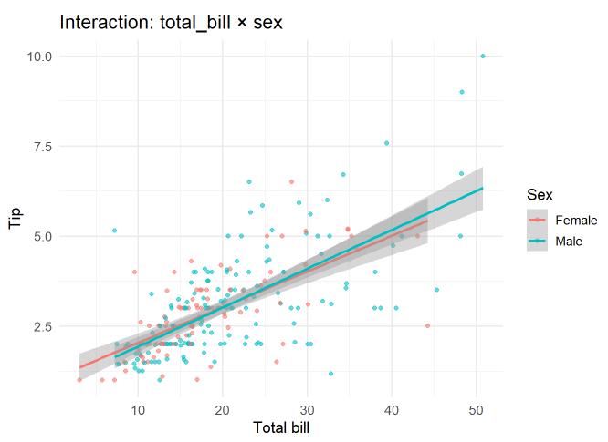
- 위 그래프 해석은 다음과 같다.
- total_bill: 유의함 → 선의 기울기 자체가 유의하게 양(+)
- sex와 total_bill:sex → 남녀 모두 총금액이 클수록 팁이 증가하는 동일한 패턴을 보이지만, 성별에 따른 기울기 차이는 통계적으로도 유의하지 않음 (p ≈ 0.58).
- 즉, 상호작용이 없다
예측선을 직접 계산해 그리기(모델 기반)
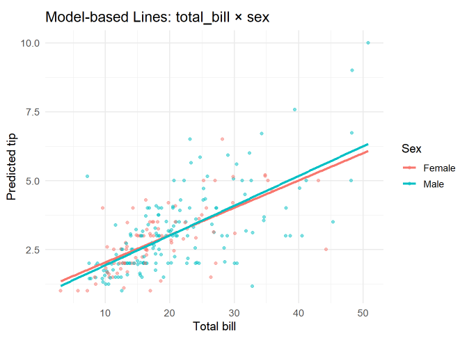
- 직접 계산해서 값을 구한 후, 시각화 하기
- total_bill의 최소~최대 값을 200개의 구간으로 나누고, sex의 두 수준(Female, Male)에 대해 조합합니다.
- 해석 결과는 동일함
grid1 <- expand.grid(
  total_bill = seq(min(tips$total_bill), max(tips$total_bill), length.out = 200),
  sex = levels(tips$sex)
)
grid1$pred <- predict(m1, newdata = grid1)

ggplot() +
  geom_point(data = tips, aes(total_bill, tip, color = sex), alpha = .5) +
  geom_line(data = grid1, aes(total_bill, pred, color = sex), size = 1.1) +
  labs(title = "Model-based Lines: total_bill × sex",
       x = "Total bill", y = "Predicted tip", color = "Sex") +
  theme_minimal(base_size = 13)
## Warning: Using `size` aesthetic for lines was deprecated in ggplot2 3.4.0.
## ℹ Please use `linewidth` instead.
## This warning is displayed once every 8 hours.
## Call `lifecycle::last_lifecycle_warnings()` to see where this warning was
## generated.
상호작용이 있는 모델
- 코드는 다음과 같다.
smoker_model <- lm(tip ~ total_bill * smoker, data = tips)
summary(smoker_model)
##
## Call:
## lm(formula = tip ~ total_bill * smoker, data = tips)
##
## Residuals:
##     Min      1Q  Median      3Q     Max
## -2.6789 -0.5238 -0.1205  0.4749  4.8999
##
## Coefficients:
##                       Estimate Std. Error t value Pr(>|t|)
## (Intercept)           0.360069   0.202058   1.782 0.076012 .
## total_bill            0.137156   0.009678  14.172  < 2e-16 ***
## smokerYes             1.204203   0.312263   3.856 0.000148 ***
## total_bill:smokerYes -0.067566   0.014189  -4.762 3.32e-06 ***
## ---
## Signif. codes:  0 '***' 0.001 '**' 0.01 '*' 0.05 '.' 0.1 ' ' 1
##
## Residual standard error: 0.9785 on 240 degrees of freedom
## Multiple R-squared:  0.506,  Adjusted R-squared:  0.4998
## F-statistic: 81.95 on 3 and 240 DF,  p-value: < 2.2e-16
계수 해석
- 계수 해석은 다음과 같다.
| 계수 항목 | 추정값(Estimate) | 표준오차(Std. Error) | p-value | 해석 |
|---|---|---|---|---|
| total_bill | 0.1372 | 0.0097 | < 0.001 | 비흡연자 그룹에서 총 결제금액이 1달러 증가할 때 팁이 약 $0.137 증가. 통계적으로 유의함. |
| smokerYes | 1.2042 | 0.3123 | 0.0001 | total_bill = 0일 때, 흡연자 그룹의 절편이 비흡연자보다 $1.204 더 큼. 통계적으로 유의함. |
| total_bill:smokerYes | -0.0676 | 0.0142 | 0.0000033 | 흡연자 그룹의 기울기가 비흡연자보다 $0.0676 작음. 즉, 결제금액 증가에 따른 팁 증가 폭이 더 완만함. |
모델 시각화
- 그래프는 다음과 같다.
grid2 <- expand.grid(
  total_bill = seq(min(tips$total_bill), max(tips$total_bill), length.out = 200),
  smoker = levels(tips$smoker)
)
grid2$pred <- predict(smoker_model, newdata = grid2)

ggplot() +
  geom_point(data = tips, aes(total_bill, tip, color = smoker), alpha = .5) +
  geom_line(data = grid2, aes(total_bill, pred, color = smoker), size = 1.1) +
  labs(title = "Model-based Lines: total_bill × smoker",
       x = "Total bill", y = "Predicted tip", color = "Smoker") +
  theme_minimal(base_size = 13)
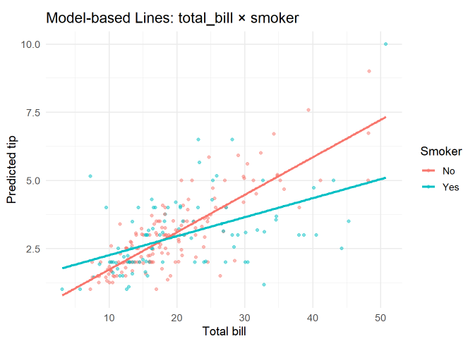
- 위 그래프 해석을 다음과 같이 할 수 있다.
| 요소 | 관찰 내용 | 해석 |
|---|---|---|
| 빨강선 (비흡연자) | 기울기가 큼 | 결제금액이 증가할수록 팁이 빠르게 증가 |
| 파랑선 (흡연자) | 절편은 높지만 기울기가 완만 | 저액 결제 시 팁이 더 높지만 고액 결제에서는 팁 증가 폭이 작음 |
| 교차점 | 약 total_bill ≈ 17~18달러 지점에서 두 선 교차 | 저액대에서는 흡연자가 팁이 더 많고, 고액대에서는 비흡연자가 더 많음 |
| 상호작용 계수 | 음(-)의 유의한 계수 (p < 0.001) | 결제금액과 팁의 관계가 흡연 여부에 따라 다르게 나타남 |
| 시각적 패턴 | 두 선이 명확히 교차 | 전형적인 상호작용 효과가 시각적으로 확인됨 |
| 해석 요약 | 그룹별 팁 증가 양상이 다름 | 팁의 기본 수준은 흡연자가 높지만, 증가율은 비흡연자가 더 큼 |
상호작용 효과의 의미
- total_bill × smoker 상호작용 계수는 유의미하게 음수(p < 0.001)였음.
- 이는 흡연자 그룹에서 결제금액이 증가할수록 팁이 증가하는 폭이 비흡연자보다 작다는 뜻.
- 팁 수준은 저액일 때는 흡연자가 높지만, 고액으로 갈수록 역전됨.