Tutorial of Ranzcr EDA
Page content
강의 홍보
- 취준생을 위한 강의를 제작하였습니다.
- 본 블로그를 통해서 강의를 수강하신 분은 게시글 제목과 링크를 수강하여 인프런 메시지를 통해 보내주시기를 바랍니다.
스타벅스 아이스 아메리카노를 선물로 보내드리겠습니다.
- [비전공자 대환영] 제로베이스도 쉽게 입문하는 파이썬 데이터 분석 - 캐글입문기

Competition
Intro
- Thanks to RANZCR/resnext50_32x4d starter [training]
- Please visit here and upvote
import os

import pandas as pd

from matplotlib import pyplot as plt
import seaborn as sns
Check File Size
- Check Each Size of Dataset Folder in this competition
- train_records = 4.5GB
- test_tfrecords = 0.5MB
- train (image data) = 6.5GB
- test (image data) = 0.8MB
import os

def get_folder_size(file_directory):
  # file_list = os.listdir(file_directory)
  dir_sizes = {}
  for r, d, f in os.walk(file_directory, False):
      size = sum(os.path.getsize(os.path.join(r,f)) for f in f+d)
      size += sum(dir_sizes[os.path.join(r,d)] for d in d)
      dir_sizes[r] = size
      print("{} is {} MB".format(r, round(size/2**20), 2))

base_dir = '../input/ranzcr-clip-catheter-line-classification'
get_folder_size(base_dir)
../input/ranzcr-clip-catheter-line-classification/test is 805 MB
../input/ranzcr-clip-catheter-line-classification/test_tfrecords is 555 MB
../input/ranzcr-clip-catheter-line-classification/train_tfrecords is 4563 MB
../input/ranzcr-clip-catheter-line-classification/train is 6592 MB
../input/ranzcr-clip-catheter-line-classification is 12524 MB
Check train file
- Let’s descirbe train
train = pd.read_csv('../input/ranzcr-clip-catheter-line-classification/train.csv', index_col = 0)
test = pd.read_csv('../input/ranzcr-clip-catheter-line-classification/sample_submission.csv', index_col = 0)
display(train.head())
display(test.head())
| ETT - Abnormal | ETT - Borderline | ETT - Normal | NGT - Abnormal | NGT - Borderline | NGT - Incompletely Imaged | NGT - Normal | CVC - Abnormal | CVC - Borderline | CVC - Normal | Swan Ganz Catheter Present | PatientID | |
|---|---|---|---|---|---|---|---|---|---|---|---|---|
| StudyInstanceUID | ||||||||||||
| 1.2.826.0.1.3680043.8.498.26697628953273228189375557799582420561 | 0 | 0 | 0 | 0 | 0 | 0 | 1 | 0 | 0 | 0 | 0 | ec89415d1 |
| 1.2.826.0.1.3680043.8.498.46302891597398758759818628675365157729 | 0 | 0 | 1 | 0 | 0 | 1 | 0 | 0 | 0 | 1 | 0 | bf4c6da3c |
| 1.2.826.0.1.3680043.8.498.23819260719748494858948050424870692577 | 0 | 0 | 0 | 0 | 0 | 0 | 0 | 0 | 1 | 0 | 0 | 3fc1c97e5 |
| 1.2.826.0.1.3680043.8.498.68286643202323212801283518367144358744 | 0 | 0 | 0 | 0 | 0 | 0 | 0 | 1 | 0 | 0 | 0 | c31019814 |
| 1.2.826.0.1.3680043.8.498.10050203009225938259119000528814762175 | 0 | 0 | 0 | 0 | 0 | 0 | 0 | 0 | 0 | 1 | 0 | 207685cd1 |
| ETT - Abnormal | ETT - Borderline | ETT - Normal | NGT - Abnormal | NGT - Borderline | NGT - Incompletely Imaged | NGT - Normal | CVC - Abnormal | CVC - Borderline | CVC - Normal | Swan Ganz Catheter Present | |
|---|---|---|---|---|---|---|---|---|---|---|---|
| StudyInstanceUID | |||||||||||
| 1.2.826.0.1.3680043.8.498.46923145579096002617106567297135160932 | 0 | 0 | 0 | 0 | 0 | 0 | 0 | 0 | 0 | 0 | 0 |
| 1.2.826.0.1.3680043.8.498.84006870182611080091824109767561564887 | 0 | 0 | 0 | 0 | 0 | 0 | 0 | 0 | 0 | 0 | 0 |
| 1.2.826.0.1.3680043.8.498.12219033294413119947515494720687541672 | 0 | 0 | 0 | 0 | 0 | 0 | 0 | 0 | 0 | 0 | 0 |
| 1.2.826.0.1.3680043.8.498.84994474380235968109906845540706092671 | 0 | 0 | 0 | 0 | 0 | 0 | 0 | 0 | 0 | 0 | 0 |
| 1.2.826.0.1.3680043.8.498.35798987793805669662572108881745201372 | 0 | 0 | 0 | 0 | 0 | 0 | 0 | 0 | 0 | 0 | 0 |
Definitions of Variables
- What’s inside data?
- StudyInstanceUID - unique ID for each image
- ETT - Abnormal - endotracheal tube placement abnormal
- ETT - Borderline - endotracheal tube placement borderline abnormal
- ETT - Normal - endotracheal tube placement normal
- NGT - Abnormal - nasogastric tube placement abnormal
- NGT - Borderline - nasogastric tube placement borderline abnormal
- NGT - Incompletely Imaged - nasogastric tube placement inconclusive due to imaging
- NGT - Normal - nasogastric tube placement borderline normal
- CVC - Abnormal - central venous catheter placement abnormal
- CVC - Borderline - central venous catheter placement borderline abnormal
- CVC - Normal - central venous catheter placement normal
- Swan Ganz Catheter Present(??)
- PatientID - unique ID for each patient in the dataset
Data Distribution of Each Variable
- why two calculations are different?
- When inserting catheters and lines into patients, some patients needs them to put on multiple positions.
- Let’s see PatientID - bf4c6da3c
- But, you realize that three groups - ETT, NGT, CVC counted seperately.
print("Total Rows of Train Data is", len(train))
print("Total Count of Each Variable in Train Data is", train.iloc[:, :-1].sum().sum())

var_cal_tmp = train.iloc[:, :-1].sum()
print(var_cal_tmp)
Total Rows of Train Data is 30083
Total Count of Each Variable in Train Data is 50619
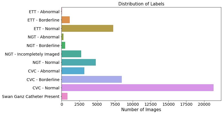
ETT - Abnormal 79
ETT - Borderline 1138
ETT - Normal 7240
NGT - Abnormal 279
NGT - Borderline 529
NGT - Incompletely Imaged 2748
NGT - Normal 4797
CVC - Abnormal 3195
CVC - Borderline 8460
CVC - Normal 21324
Swan Ganz Catheter Present 830
dtype: int64
train.iloc[1].to_frame().T
| ETT - Abnormal | ETT - Borderline | ETT - Normal | NGT - Abnormal | NGT - Borderline | NGT - Incompletely Imaged | NGT - Normal | CVC - Abnormal | CVC - Borderline | CVC - Normal | Swan Ganz Catheter Present | PatientID | |
|---|---|---|---|---|---|---|---|---|---|---|---|---|
| 1.2.826.0.1.3680043.8.498.46302891597398758759818628675365157729 | 0 | 0 | 1 | 0 | 0 | 1 | 0 | 0 | 0 | 1 | 0 | bf4c6da3c |
Quick Visualization
- In general, CVC outnumbered other group.
fig, ax = plt.subplots(figsize=(10, 6))
sns.barplot(x = var_cal_tmp.values, y = var_cal_tmp.index, ax=ax)
ax.tick_params(axis="x", labelsize=14)
ax.tick_params(axis="y", labelsize=14)
ax.set_xlabel("Number of Images", fontsize=15)
ax.set_title("Distribution of Labels", fontsize=15)
Text(0.5, 1.0, 'Distribution of Labels')
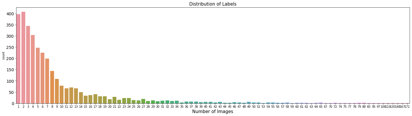
- The number of Patients are smaller than total data.
- It means some patients are frequently checked, depending upon patients
print("Number of Unique Patients: ", train["PatientID"].unique().shape[0])
print("Number of Total Data: ", len(train["PatientID"]))
Number of Unique Patients:  3255
Number of Total Data:  30083
tmp = train['PatientID'].value_counts()
print(tmp)
fig, ax = plt.subplots(figsize=(24, 6))
sns.countplot(x = tmp.values, ax=ax)
ax.tick_params(axis="x", labelsize=10)
ax.tick_params(axis="y", labelsize=14)
ax.set_xlabel("Number of Images", fontsize=15)
ax.set_title("Distribution of Labels", fontsize=15)
05029c63a    172
55073fece    167
26da0d5ad    148
8849382d0    130
34242119f    110
            ...
ad32e88e0      1
7755053cb      1
2d5a5f0d0      1
1951dc11c      1
22e8f333f      1
Name: PatientID, Length: 3255, dtype: int64


Text(0.5, 1.0, 'Distribution of Labels')
- Now, we need to see the distribution of data in each variable.
target_cols = ['ETT - Abnormal', 'ETT - Borderline', 'ETT - Normal', 'NGT - Abnormal',
               'NGT - Borderline', 'NGT - Incompletely Imaged', 'NGT - Normal', 'CVC - Abnormal',
               'CVC - Borderline', 'CVC - Normal', 'Swan Ganz Catheter Present']

fig, ax = plt.subplots(4, 3, figsize=(16, 10))
for i, col in enumerate(train[target_cols].columns[0:]):
  print(i, col)
  if i <= 2:
    ax[0, i].hist(train[col].values)
    ax[0, i].set_title(f'target: {col}')
  elif i <= 5:
    ax[1, i-3].hist(train[col].values)
    ax[1, i-3].set_title(f'target: {col}')
  elif i <= 8:
    ax[2, i-6].hist(train[col].values)
    ax[2, i-6].set_title(f'target: {col}')
  else:
    ax[3, i-9].hist(train[col].values)
    ax[3, i-9].set_title(f'target: {col}')

fig.tight_layout()
fig.subplots_adjust(top=0.95)
0 ETT - Abnormal
1 ETT - Borderline
2 ETT - Normal
3 NGT - Abnormal
4 NGT - Borderline
5 NGT - Incompletely Imaged
6 NGT - Normal
7 CVC - Abnormal
8 CVC - Borderline
9 CVC - Normal
10 Swan Ganz Catheter Present
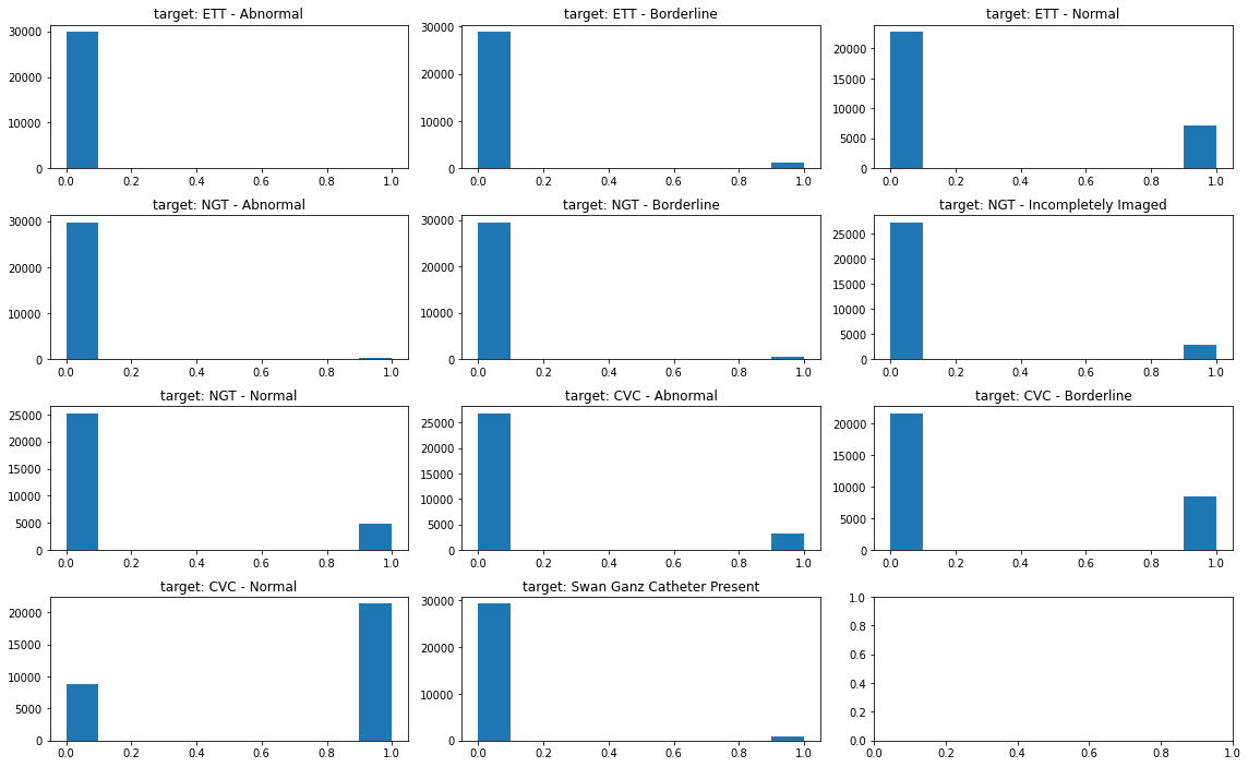
- How to interpret the graph?
- CVC group is the top most amongst groups
- In each group, Normal is the top most.
- This datasets are typically imbalanced, and multi-classification problem is revealed.
Background Knowledge
- Since my major is far from this medical area, it difficults to figure what to classify from images.
- So, need some videos to understand the processing.
- Thanks to RANZCR CLiP: Visualize and Understand Dataset
- Please visit here and upvote
Endotracheal Tube
- It’s so called ETT in this dataset.
from IPython.display import YouTubeVideo
YouTubeVideo('FtJr7i7ENMY')
Nasogastric Tube
- It’s so called NTT in this dataset.
YouTubeVideo('Abf3Gd6AaZQ')
Central venous catheter
- It’s so called CVC in this dataset.
YouTubeVideo('mTBrCMn86cU')
Swan Ganz Catheter Present
- It’s Swan Ganz Catheter Present
YouTubeVideo('YkN30T6ig30')
Check train annotation file
- What’s Inside train_annotations file?
- The main purpose is said that ‘These are segmentation annotations for training samples that have them. They are included solely as additional information for competitors.’
- Let’s look at data
annot = pd.read_csv("../input/ranzcr-clip-catheter-line-classification/train_annotations.csv")
annot.head(10)
| StudyInstanceUID | label | data | |
|---|---|---|---|
| 0 | 1.2.826.0.1.3680043.8.498.12616281126973421762... | CVC - Normal | [[1487, 1279], [1477, 1168], [1472, 1052], [14... |
| 1 | 1.2.826.0.1.3680043.8.498.12616281126973421762... | CVC - Normal | [[1328, 7], [1347, 101], [1383, 193], [1400, 2... |
| 2 | 1.2.826.0.1.3680043.8.498.72921907356394389969... | CVC - Borderline | [[801, 1207], [812, 1112], [823, 1023], [842, ... |
| 3 | 1.2.826.0.1.3680043.8.498.11697104485452001927... | CVC - Normal | [[1366, 961], [1411, 861], [1453, 751], [1508,... |
| 4 | 1.2.826.0.1.3680043.8.498.87704688663091069148... | NGT - Normal | [[1862, 14], [1845, 293], [1801, 869], [1716, ... |
| 5 | 1.2.826.0.1.3680043.8.498.87704688663091069148... | CVC - Normal | [[906, 604], [1103, 578], [1242, 607], [1459, ... |
| 6 | 1.2.826.0.1.3680043.8.498.87704688663091069148... | ETT - Normal | [[1781, 804], [1801, 666], [1791, 496], [1798,... |
| 7 | 1.2.826.0.1.3680043.8.498.53113362093090654004... | CVC - Normal | [[1152, 938], [1193, 856], [1265, 795], [1362,... |
| 8 | 1.2.826.0.1.3680043.8.498.83331936392921199432... | NGT - Normal | [[1903, 73], [1934, 768], [1917, 1061], [1866,... |
| 9 | 1.2.826.0.1.3680043.8.498.83331936392921199432... | CVC - Normal | [[92, 1857], [163, 1936], [251, 1917], [282, 1... |
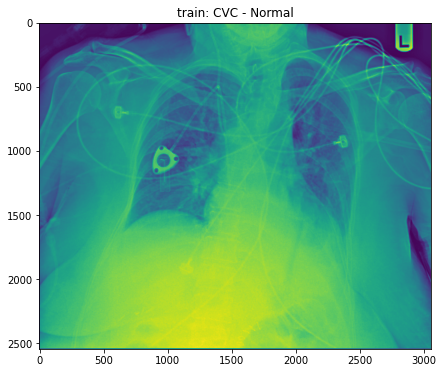
Visualization of X-rays image
- combined train + train_annotations, let’s draw sample image
from PIL import Image, ImageDraw

def train_base_chest_plot(row_ind, base_dir):
    row = annot.loc[row_ind]
    train_img = Image.open(base_dir + row['StudyInstanceUID'] + '.jpg')
    uid = row['StudyInstanceUID']
    label = row['label']
    fig, ax = plt.subplots(figsize=(15, 6))
    ax.imshow(train_img)
    plt.title(f"train: {label}")

base_dir = '../input/ranzcr-clip-catheter-line-classification/train/'
train_base_chest_plot(1, base_dir)
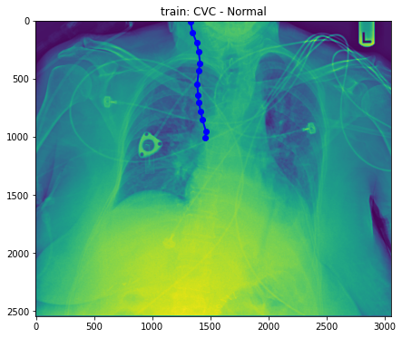
- But, what we need is to draw tube. Thus, we need to use column ‘data’ in this plot. Let’s do this.
import ast
import numpy as np
def train_base_tube_plot(row_ind, base_dir):
row = annot.loc[row_ind]
train_img = Image.open(base_dir + row['StudyInstanceUID'] + '.jpg')
uid = row['StudyInstanceUID']
label = row['label']
data = np.array(ast.literal_eval(row['data']))
fig, ax = plt.subplots(figsize=(15, 6))
ax.imshow(train_img)
ax.plot(data[:, 0], data[:, 1], color = 'b', linewidth=2, marker='o')
plt.title(f"train: {label}")
base_dir = '../input/ranzcr-clip-catheter-line-classification/train/'
train_base_tube_plot(1, base_dir)
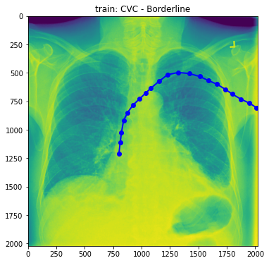
train_base_tube_plot(2, base_dir)
train_base_tube_plot(25, base_dir)
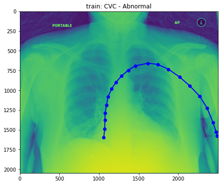
- Well, still difficult to figure out what the difference between normal and abnormal is. So, Droped to draw more.