Pandas

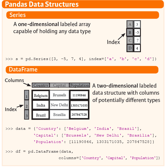
Pandas Data Handling 1편

강의 홍보

I. Kaggle에서 타이타닉 데이터 가져오기

  • 캐글 데이터 가져오는 예제는 본 Kaggle with Google Colab에서 참고하기를 바란다.
  • 먼저 kaggle 패키지를 설치한다.
!pip install kaggle
Requirement already satisfied: kaggle in /usr/local/lib/python3.6/dist-packages (1.5.6)
Requirement already satisfied: urllib3<1.25,>=1.21.1 in /usr/local/lib/python3.6/dist-packages (from kaggle) (1.24.3)
Requirement already satisfied: six>=1.10 in /usr/local/lib/python3.6/dist-packages (from kaggle) (1.12.0)
Requirement already satisfied: python-dateutil in /usr/local/lib/python3.6/dist-packages (from kaggle) (2.8.1)
Requirement already satisfied: tqdm in /usr/local/lib/python3.6/dist-packages (from kaggle) (4.41.1)
Requirement already satisfied: python-slugify in /usr/local/lib/python3.6/dist-packages (from kaggle) (4.0.0)
Requirement already satisfied: certifi in /usr/local/lib/python3.6/dist-packages (from kaggle) (2020.6.20)
Requirement already satisfied: requests in /usr/local/lib/python3.6/dist-packages (from kaggle) (2.23.0)
Requirement already satisfied: text-unidecode>=1.3 in /usr/local/lib/python3.6/dist-packages (from python-slugify->kaggle) (1.3)
Requirement already satisfied: chardet<4,>=3.0.2 in /usr/local/lib/python3.6/dist-packages (from requests->kaggle) (3.0.4)
Requirement already satisfied: idna<3,>=2.5 in /usr/local/lib/python3.6/dist-packages (from requests->kaggle) (2.9)
  • kaggle 인증키를 업로드 하여 권한 부여 한다.
from google.colab import files
files.upload()
Saving kaggle.json to kaggle.json


{'kaggle.json': b'{"username":"j2hoon85","key":"5a23c8dba5a151100b483a587eafdac8"}'}
!mkdir -p ~/.kaggle # 파일 생성
!mv kaggle.json ~/.kaggle/ # kaggle.json 파일 이동
!chmod 600 ~/.kaggle/kaggle.json # 권한 부여
!kaggle competitions list
Warning: Looks like you're using an outdated API Version, please consider updating (server 1.5.6 / client 1.5.4)
ref                                            deadline             category            reward  teamCount  userHasEntered  
---------------------------------------------  -------------------  ---------------  ---------  ---------  --------------  
tpu-getting-started                            2030-06-03 23:59:00  Getting Started      Kudos        125           False  
digit-recognizer                               2030-01-01 00:00:00  Getting Started  Knowledge       2958           False  
titanic                                        2030-01-01 00:00:00  Getting Started  Knowledge      22881            True  
house-prices-advanced-regression-techniques    2030-01-01 00:00:00  Getting Started  Knowledge       4985            True  
connectx                                       2030-01-01 00:00:00  Getting Started  Knowledge        673           False  
nlp-getting-started                            2030-01-01 00:00:00  Getting Started      Kudos       1455            True  
competitive-data-science-predict-future-sales  2020-12-31 23:59:00  Playground           Kudos       7626           False  
halite                                         2020-09-15 23:59:00  Featured              Swag        534           False  
birdsong-recognition                           2020-09-15 23:59:00  Research           $25,000        244           False  
landmark-retrieval-2020                        2020-08-17 23:59:00  Research           $25,000         53           False  
siim-isic-melanoma-classification              2020-08-17 23:59:00  Featured           $30,000       1672           False  
global-wheat-detection                         2020-08-04 23:59:00  Research           $15,000       1353           False  
open-images-object-detection-rvc-2020          2020-07-31 16:00:00  Playground       Knowledge         45           False  
open-images-instance-segmentation-rvc-2020     2020-07-31 16:00:00  Playground       Knowledge          9           False  
hashcode-photo-slideshow                       2020-07-27 23:59:00  Playground       Knowledge         50           False  
prostate-cancer-grade-assessment               2020-07-22 23:59:00  Featured           $25,000        765           False  
alaska2-image-steganalysis                     2020-07-20 23:59:00  Research           $25,000        869           False  
m5-forecasting-accuracy                        2020-06-30 23:59:00  Featured           $50,000       5558            True  
m5-forecasting-uncertainty                     2020-06-30 23:59:00  Featured           $50,000        909           False  
trends-assessment-prediction                   2020-06-29 23:59:00  Research           $25,000       1047           False  
  • 캐글에서 데이터를 내려받는다.
!kaggle competitions download -c titanic
Warning: Looks like you're using an outdated API Version, please consider updating (server 1.5.6 / client 1.5.4)
gender_submission.csv: Skipping, found more recently modified local copy (use --force to force download)
test.csv: Skipping, found more recently modified local copy (use --force to force download)
train.csv: Skipping, found more recently modified local copy (use --force to force download)
!ls
chloevan_key.pem  gender_submission.csv  sample_data  test.csv	train.csv
  • 이제, 판다스를 활용해서 데이터를 불러온다.
import pandas as pd

titanic_df = pd.read_csv(r'train.csv')
titanic_df.head(3)
print('titanic 변수 type:', type(titanic_df))
titanic 변수 type: <class 'pandas.core.frame.DataFrame'>

II. 데이터 핸들링을 위한 주요 함수 소개

  • 본 장에서는 데이터 핸들링을 위한 몇가지 주요함수를 소개한다.

(1) value_counts()

  • value_counts()는 해당 칼럼값의 데이터 유형과 건수를 반환함
val_count = titanic_df['Embarked'].value_counts()
print(type(val_count))
print(val_count)
<class 'pandas.core.series.Series'>
S    644
C    168
Q     77
Name: Embarked, dtype: int64

(2) 데이터프레임 일부 삭제

  • drop()axis의 기준에 따라서 행과 열의 데이터를 삭제한다.
  • 이 때, 주요 파라미터는 labels, inplace, axis에 따라 구분된다.
    • labels: 컬럼명 또는 행의 인덱스
    • inplace: 데이터 업데이트
    • axis: 0은 행 방향, 1은 컬럼 방향
  • axis=1를 활용하여 우선 컬럼명을 삭제한다.
data = titanic_df.copy()
data_drop = data.drop(labels = 'Age', axis=1)
data_drop.head()

<

EDA with Pandas - Data Merge

강의 홍보

I. 개요

  • 실무 데이터에서는 여러가지 데이터를 만나는 경우가 흔하다.
  • 이 때, SQL에서 데이터를 직접 병합하는 방법이 좋다.
  • 그러나, 현실적으로 DB에 접근하는 권한을 가진 경우는 흔하지는 않다. 현재 운영중인 서비스상에 DB를 직접 만지는 경우는 거의 없다 (DBA가 할지도..)
  • 따라서, 데이터분석가는 흩어져 있는 데이터 Dump를 받게 될 가능성이 큰데, 이 때 Python에서 데이터를 병합하는 작업을 진행하게 된다.
  • Kaggle이나 각종 경진대회에 출전하게 되면 서로 다른 데이터를 합쳐야 하는 경우가 매우 많다.

II. 모듈 Import

import pandas as pd
print(pd.__version__)
1.0.4
  • 데이터프레임을 보다 이쁘게 출력하기 위해 다음 2개의 패키지를 불러온다.
from IPython.core.display import display, HTML
from tabulate import tabulate

III. Pandas 데이터 병합 Sample Tutorial

  • 간단하게 데이터를 병합하는 방법에 대해 실습을 진행한다.

(1) 파라미터 세팅

  • 먼저, 행과 열을 최대 출력하는 개수를 지정한다.
pd.set_option('display.max_columns', 500)
pd.set_option('display.max_rows', 500)

(2) 데이터 생성

  • 먼저 가상의 데이터를 두개 만든다.
temp_1 = pd.DataFrame({'key': ['A', 'B', 'C', 'D'], 
                       'num1': [1,2,3,4]})
print(tabulate(temp_1, headers=['key', 'num'], tablefmt='pipe'))
|    | key   |   num |
|---:|:------|------:|
|  0 | A     |     1 |
|  1 | B     |     2 |
|  2 | C     |     3 |
|  3 | D     |     4 |
temp_2 = pd.DataFrame({'key': ['A', 'B', 'E', 'F'], 
                       'num2': [5,6,7,8]})
print(tabulate(temp_2, headers=['key', 'num'], tablefmt='pipe'))
|    | key   |   num |
|---:|:------|------:|
|  0 | A     |     5 |
|  1 | B     |     6 |
|  2 | E     |     7 |
|  3 | F     |     8 |

(3) Data Merge - inner join

  • key값을 근거로 데이터를 병합한다.
  • 이 때, merge의 형태는 inner join 형태로 출력된다.
merge_df = pd.merge(temp_1, temp_2, on='key')
print(tabulate(merge_df, headers=['key', 'num1', 'num2'], tablefmt='pipe'))
|    | key   |   num1 |   num2 |
|---:|:------|-------:|-------:|
|  0 | A     |      1 |      5 |
|  1 | B     |      2 |      6 |
inner_df = pd.merge(temp_1, temp_2, on='key', how='inner')
print(tabulate(inner_df, headers=['key', 'num1', 'num2'], tablefmt='pipe'))
|    | key   |   num1 |   num2 |
|---:|:------|-------:|-------:|
|  0 | A     |      1 |      5 |
|  1 | B     |      2 |      6 |
  • 위 두개의 결과값이 똑같음을 확인할 수 있다.

(4) Data Merge - outer join

  • 이번에는 outer join을 해보자.
outer_df = pd.merge(temp_1, temp_2, on='key', how='outer')
print(tabulate(outer_df, headers=['key', 'num1', 'num2'], tablefmt='pipe'))
|    | key   |   num1 |   num2 |
|---:|:------|-------:|-------:|
|  0 | A     |      1 |      5 |
|  1 | B     |      2 |      6 |
|  2 | C     |      3 |    nan |
|  3 | D     |      4 |    nan |
|  4 | E     |    nan |      7 |
|  5 | F     |    nan |      8 |
  • 결과값을 보면, 우선 key값은 모두 출력되었다.
  • 이 때, 각 데이터에서 가져오는 num1num2Column도 같이 들어오는데, 각 column마다 없는 값들은 이렇게 nan으로 조회됨을 확인할 수 있다.

(5) Assignment

  • 이제 수강생 분들이 left & right 조인을 해보도록 한다.
  • 공식문서를 보면서 코드 작성하는 것을 추천한다.
# pd.merge(temp_1, temp_2) 여기 코드에서 남은 코드를 작성하면 됩니다. 
right_df = pd.merge(temp_1, temp_2, on='key', how='left')
print(tabulate(right_df, headers=['key', 'num1', 'num2'], tablefmt='pipe'))
|    | key   |   num1 |   num2 |
|---:|:------|-------:|-------:|
|  0 | A     |      1 |      5 |
|  1 | B     |      2 |      6 |
|  2 | E     |    nan |      7 |
|  3 | F     |    nan |      8 |
  • 그리고 이번에는 left join을 해본다.
# pd.merge(temp_1, temp_2) 여기 코드에서 남은 코드를 작성하면 됩니다. 
right_df = pd.merge(temp_1, temp_2, on='key', how='left')
print(tabulate(right_df, headers=['key', 'num1', 'num2'], tablefmt='pipe'))
|    | key   |   num1 |   num2 |
|---:|:------|-------:|-------:|
|  0 | A     |      1 |      5 |
|  1 | B     |      2 |      6 |
|  2 | C     |      3 |    nan |
|  3 | D     |      4 |    nan |

VI. What’s next

  • 데이터를 병합하는 방법 중 Merge에 대해서 배웠다.
  • Merge에는 크게 4가지 방법이 있고, 방법에 따라서 최종 데이터의 출력값이 서로 다름을 확인하였다.
  • 다음 시간에는 또다른 병합 방법인 Concatenate에 학습하도록 한다.

EDA with Python - Pandas

강의 홍보

I. 개요

  • Pandaspanel data의 의미를 가지고 있다.
  • 흔히, 엑셀 데이터로 불리우는 관계형(Relational) 또는 레이블링된(Labeling)된 데이터를 보다 쉽게, 직관적으로 작업할 수 있도록 설계되어 있다.
  • Python에서 데이터 분석을 수행하기 위한 매우 기초적이며 높은 수준의 문법을 제공한다.
  • Pandas는 크게 Series & DataFrame을 다룰 수 있도록 기초 문법을 제공하고 있다.
  • Pandas가 다루는 여러 종류의 데이터를 확인해보자.
    • SQL 테이블 또는 Excel 스프레드시트에서와 같이 형식의 행과 열이 있는 표 형식 데이터
    • 순서 및 순서 지정되지 않은(고정 빈도일 필요는 없음) 시계열 데이터.
    • 행 및 열 레이블이 있는 임의 행렬 데이터(동일하게 입력 또는 이기종)
    • 기타 형태의 관측/통계 데이터 세트

II. 모듈 Import

import pandas as pd
print(pd.__version__)
1.0.3

III. Pandas 기본 활용법

  • Pandas가 제공하는 다양한 기능은 다음과 같지만, 본 튜토리얼에서는 Sample 위주로 다루도록 한다.
    • 부동 소수점 데이터뿐만 아니라 부동 소수점 데이터에서도 결측 데이터(NaN으로 표시됨)를 쉽게 처리함
    • 크기 변이성: DataFrame 및 고차원 객체에서 열을 삽입 및 삭제 가능
    • 자동 및 명시적 데이터 정렬: 객체를 라벨 집합에 명시적으로 정렬하거나, 사용자가 라벨을 무시하고 Series, DataFrame 등이 자동으로 데이터를 계산에서 정렬 가능
    • 데이터 집합에서 데이터 집합의 분할 적용 결합 작업을 수행할 수 있는 기능
    • 다른 PythonNumPy 데이터 구조에서 색인이 다른 데이터를 DataFrame 개체로 쉽게 변환
    • 지능형 라벨 기반 슬라이싱, 고급 인덱싱 및 대용량 데이터 세트 부분 집합 취하기
    • 직관적인 데이터 세트 병합 및 결합
    • 유연한 데이터 세트 재구성 및 피벗테이블 구성
    • 축의 계층적 라벨링(눈금당 여러 개의 라벨을 가질 수 있음)
    • 플랫 파일(CSV 및 구분), Excel 파일, 데이터베이스 로딩 및 초고속 HDF5 형식의 데이터 저장/로딩에 사용되는 강력한 데이터 IO 도구
    • 시계열별 기능: 날짜 범위 생성 및 주파수 변환, 이동 창 통계, 날짜 이동 및 지연.

IV. Pandas Sample Tutorial

  • 간단하게 Pandas를 활용한 Tutorial을 확인해보자.

(1) 파라미터 세팅

  • 먼저, 행과 열을 최대 출력하는 개수를 지정한다.
pd.set_option('display.max_columns', 500)
pd.set_option('display.max_rows', 500)

(2) 데이터 생성

  • 데이터를 생성하는 방법은 크게 2가지로 구분된다. (Series, DataFrame)
  • 먼저 Series를 만들어보자.
temp_series = pd.Series([1,2,3,5,8,13,21])
print(temp_series)
0     1
1     2
2     3
3     5
4     8
5    13
6    21
dtype: int64
  • 이제 Series에 있는 데이터와 함께 DataFrame을 만든다.
series_df = pd.DataFrame({
    "No":range(1,5), 
    "날짜":pd.Timestamp('20200601'), 
    "출석점수":pd.Series(5, index=list(range(4)), dtype='float64'), 
    "등급":pd.Categorical(["A등급", "B등급", "C등급", "D등급"]), 
    "구분":"학점"
})

print(series_df)
   No         날짜  출석점수   등급  구분
0   1 2020-06-01   5.0  A등급  학점
1   2 2020-06-01   5.0  B등급  학점
2   3 2020-06-01   5.0  C등급  학점
3   4 2020-06-01   5.0  D등급  학점
  • 이번에는 딕셔너리에서 데이터프레임으로 변환하는 소스코드다.
  • 아래 코드에서 보여주고자 하는 것은 딕셔너리의 크기가 동일하지 않아도, 데이터프레임으로 변환되는데 문제가 없다.
  • 다만, NaN으로 채울 뿐이다.
dict_df = [{'가': '사과', '나': '볼'},{'가': '비행기', '나': '방망이', '다': '고양이'}]
dict_df = pd.DataFrame(dict_df)
print(dict_df)
     가    나    다
0   사과    볼  NaN
1  비행기  방망이  고양이
  • 이번에는 배열에서 데이터프레임으로 변환하는 소스코드다.
sdf = {
    '국가':['한국', '미국', '일본'],
    'ISO-Code':[1,2,3],
    '지역': [4180.69, 4917.94, 454.07,],
    '위치': ["서울", "LA", "동경"]
    }
sdf = pd.DataFrame(sdf)
print(sdf)
   국가  ISO-Code       지역  위치
0  한국         1  4180.69  서울
1  미국         2  4917.94  LA
2  일본         3   454.07  동경

(3) 파일 입출력

  • 외부 데이터의 파일 입출력에 대한 코드를 입력한다.
url = 'http://archive.ics.uci.edu/ml/machine-learning-databases/adult/adult.data'
df = pd.read_csv(url)
print(df.head(2))
   39          State-gov   77516   Bachelors   13        Never-married  \
0  50   Self-emp-not-inc   83311   Bachelors   13   Married-civ-spouse   
1  38            Private  215646     HS-grad    9             Divorced   

         Adm-clerical   Not-in-family   White   Male   2174   0   40  \
0     Exec-managerial         Husband   White   Male      0   0   13   
1   Handlers-cleaners   Not-in-family   White   Male      0   0   40   

    United-States   <=50K  
0   United-States   <=50K  
1   United-States   <=50K  
  • 컬럼명이 지정되지 않아 관측값이 컬럼명 위치에 있는 것을 확인할 수 있다.
  • 이 때에는 컬럼명을 먼저 저장한 뒤, 아래와 같은 코드로 실행하면 정상적으로 데이터프레임이 완성된다.
columns = ['age', 'workclass', 'fnlwgt', 'education', 'education_num', 
           'marital_status', 'occupation', 'relationship', 'ethnicity', 
           'gender','capital_gain','capital_loss','hours_per_week','country_of_origin','income']

df2 = pd.read_csv(url, names=columns)
print(df2.head(2))
   age          workclass  fnlwgt   education  education_num  \
0   39          State-gov   77516   Bachelors             13   
1   50   Self-emp-not-inc   83311   Bachelors             13   

        marital_status        occupation    relationship ethnicity gender  \
0        Never-married      Adm-clerical   Not-in-family     White   Male   
1   Married-civ-spouse   Exec-managerial         Husband     White   Male   

   capital_gain  capital_loss  hours_per_week country_of_origin  income  
0          2174             0              40     United-States   <=50K  
1             0             0              13     United-States   <=50K  
  • 컬럼명에 대한 정보는 Adult Data Set 에서 참고한다.
  • 판다스를 배울 때 조금더 자세히 배우겠지만, info() 함수를 사용하면 데이터의 일반적인 정보를 확인할 수 있다.
print(df2.info())
<class 'pandas.core.frame.DataFrame'>
RangeIndex: 32561 entries, 0 to 32560
Data columns (total 15 columns):
 #   Column             Non-Null Count  Dtype 
---  ------             --------------  ----- 
 0   age                32561 non-null  int64 
 1   workclass          32561 non-null  object
 2   fnlwgt             32561 non-null  int64 
 3   education          32561 non-null  object
 4   education_num      32561 non-null  int64 
 5   marital_status     32561 non-null  object
 6   occupation         32561 non-null  object
 7   relationship       32561 non-null  object
 8   ethnicity          32561 non-null  object
 9   gender             32561 non-null  object
 10  capital_gain       32561 non-null  int64 
 11  capital_loss       32561 non-null  int64 
 12  hours_per_week     32561 non-null  int64 
 13  country_of_origin  32561 non-null  object
 14  income             32561 non-null  object
dtypes: int64(6), object(9)
memory usage: 3.7+ MB
None

V. 결론

  • 간단하게 Pandas를 활용한 데이터 생성 및 파일 입출력에 대해서 배우는 시간을 가졌다.
  • 만약, 빠르게 판다스를 활용하여 데이터 전처리를 연습 하고 싶다면, 공식홈페이지에 있는 10 minutes to pandas에서 학습하는 것을 권장한다.
  • 강사는 Kaggle 데이터를 활용하여 Pandas 함수를 응용할 것이다.

Reference

Mukhiya, Suresh Kumar, and Usman Ahmed. “Hands-On Exploratory Data Analysis with Python.” Packt Publishing, Mar. 2020, www.packtpub.com/data/hands-on-exploratory-data-analysis-with-python.

Pandas Lambda Apply 함수 활용

강의 홍보

I. Iterrows, Itertuples 복습

이번 포스팅은 For-loop의 대안에 관한 함수 apply에 관한 내용이다. 본 포스트를 보고 학습하시기 전에 Pandas Iterrows 함수 활용Pandas Itertuples 함수 활용에서 학습 하기를 바란다.

지난시간과 마찬가지로 데이터는 동일한 것을 쓰도록 한다.

Pandas Itertuples 함수 활용

강의 홍보

I. Iterrows

이번 포스팅은 Iterrows()의 확장개념입니다. 본 포스트를 보고 학습하시기 전에 Pandas Iterrows 함수 활용에서 학습 하기를 바란다.

II. Itertuples의 개념

itertuples()는 기본적으로 iterrows() 함수보다는 빠르다.

import pandas as pd
import io
import requests
import pprint

url = 'https://raw.githubusercontent.com/chloevan/datasets/master/sports/baseball_stats.csv'
url=requests.get(url).content
baseball_stats = pd.read_csv(io.StringIO(url.decode('utf-8')))

pprint.pprint(baseball_stats.head())
  Team League  Year   RS   RA   W   OBP   SLG    BA  Playoffs  RankSeason  \
0  ARI     NL  2012  734  688  81  0.33  0.42  0.26         0         NaN   
1  ATL     NL  2012  700  600  94  0.32  0.39  0.25         1         4.0   
2  BAL     AL  2012  712  705  93  0.31  0.42  0.25         1         5.0   
3  BOS     AL  2012  734  806  69  0.32  0.41  0.26         0         NaN   
4  CHC     NL  2012  613  759  61  0.30  0.38  0.24         0         NaN   

   RankPlayoffs    G  OOBP  OSLG  
0           NaN  162  0.32  0.41  
1           5.0  162  0.31  0.38  
2           4.0  162  0.32  0.40  
3           NaN  162  0.33  0.43  
4           NaN  162  0.34  0.42  

III. 조건부 행 추출

드디어 Python 데이터 분석가로 보스턴 레드박스(BOS)야구팀에 취직을 했다고 가정을 해보자. 단장이 2008 ~ 2010년까지의 득점과 실점의 차이를 보고 싶다고 요청을 해왔다. 이럴 때 어떻게 해야 할까?