SQLitebroswer 설치 (M1, Mac)

개요

• SQLitebroswer 설치를 진행해본다.

설치

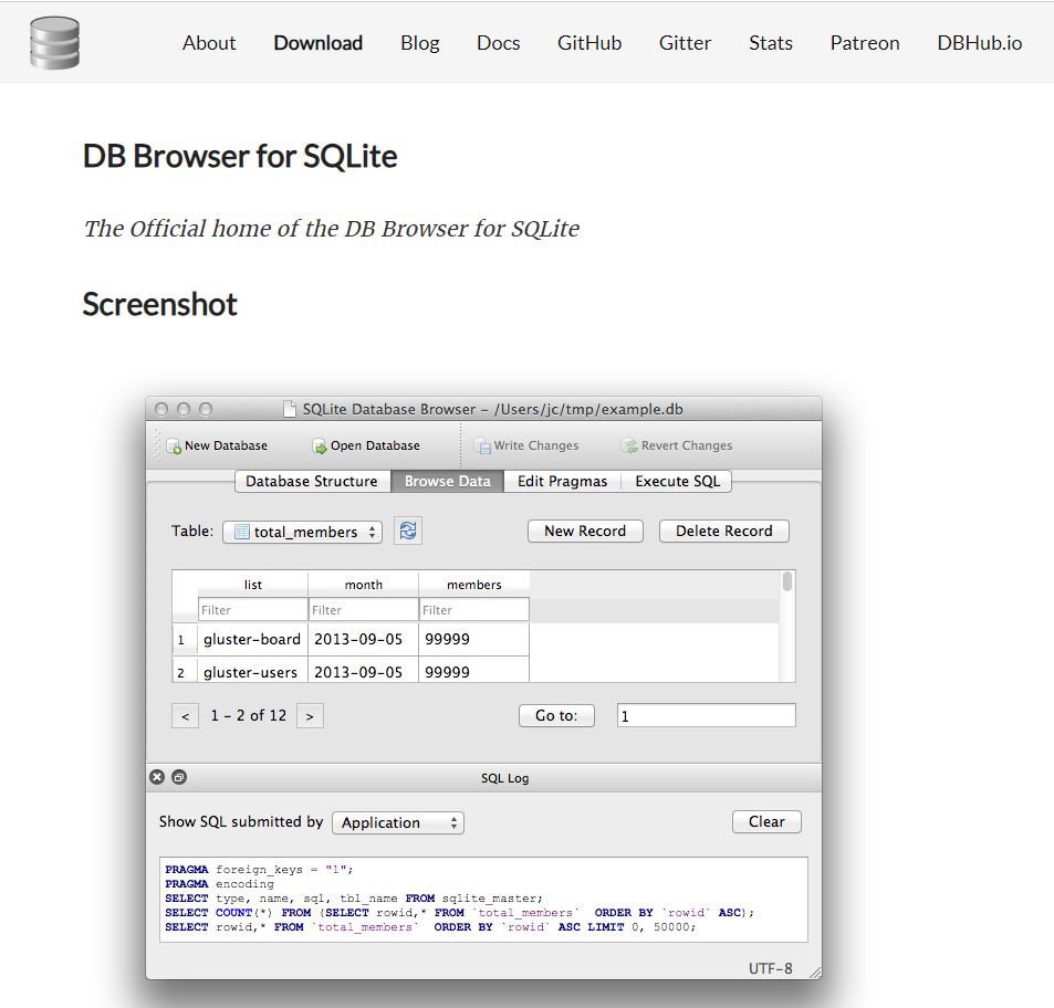
• 주소 : https://sqlitebrowser.org/
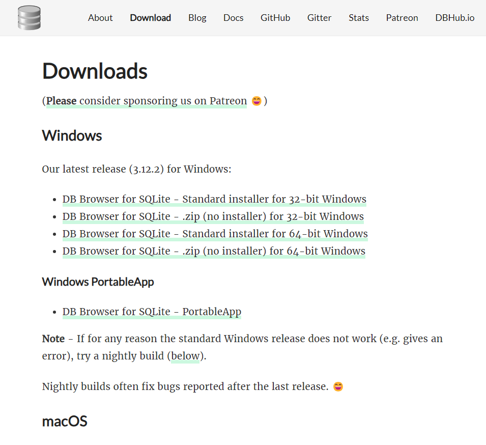
• Download 버튼을 클릭한다.

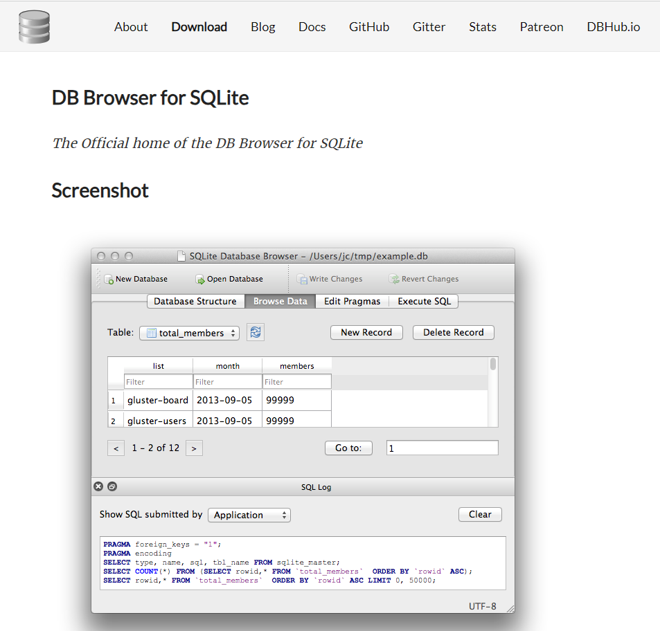
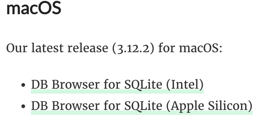
• 자신의 OS에 맞는 버전을 선택해 다운로드 후 설치
• 필자는 Apple Silicon 버전을 선택했다.

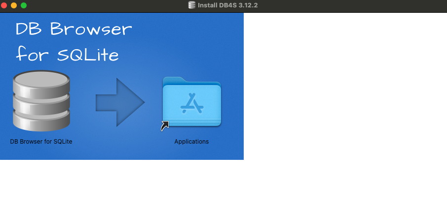
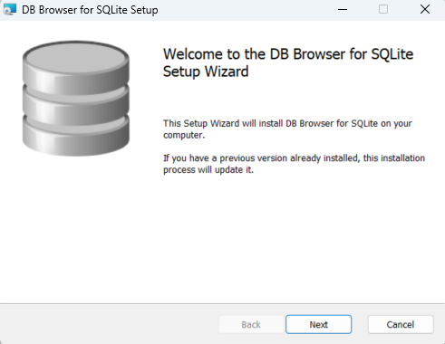
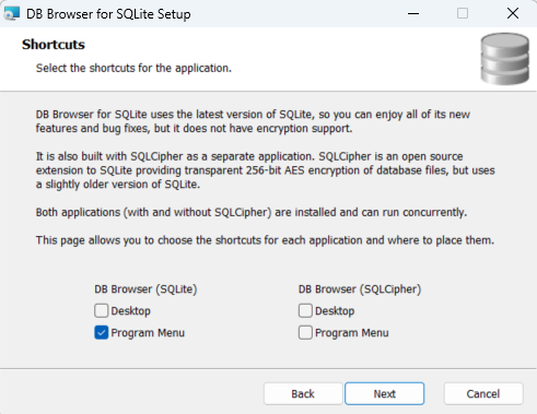
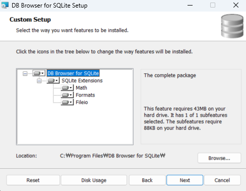
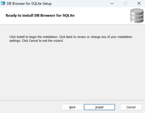
• 아래 그림과 같이 추가하면 된다.

개요

• SQLitebroswer 설치를 진행해본다.

설치

• 주소 : https://sqlitebrowser.org/
• Download 버튼을 클릭한다.

• 자신의 OS에 맞는 버전을 선택해 다운로드 후 설치
• 필자는 Standard installer for 64-bit Windows 다운로드 받았다.

• 설치 프로그램을 실행한 후, 아래와 같이 순차적으로 실행한다.

끝.

개요

• 캐글에서 한글폰트를 적용하는 방법에 대해 알아본다.
• 가장 간편한 방법은 폰트를 업로드 한 뒤 업데이트 하는 방식이다.

폰트 확인

• 폰트는 아래 사이트에서 다운로드 받는다.
• 사이트 : https://hangeul.naver.com/font
• 여기에서 나눔글꼴을 다운로드 받았다.

폰트 압축풀기

• 다운로드 폰트를 압축 풀기 하면 매우 다양한 폰트가 확인이 된다.
• 여기에서 나눔스퀘어 > NanumFontSetup_TTF_SQUARE 파일에서 폰트 목록을 확인한다.

폰트 업로드

• 이제 현재 사용하는 캐글 노트북에 추가한다.
• 임의의 font 폴더명을 입력했다.

• Create 버튼을 클릭한다.

• 업로드 이후에 폴더에 폰트가 들어간 것을 확인한다.

개요

• statsmodels를 활용하여 범주형 데이터가 포함된 회귀식을 산정해본다.
• 범주형 데이터의 특정 값을 변동하는 방법을 배운다.
• 더불어서 R로 간단한 회귀식도 만들어보자!

강의소개

• 인프런에서 Streamlit 관련 강의를 진행하고 있습니다.
• 인프런 : https://inf.run/YPniH

라이브러리 확인

• statsmodels의 라이브러리는 현재 0.14.1 버전이다.
  • 라이브러리 참조 : https://www.statsmodels.org/stable/index.html

import statsmodels
import seaborn as sns 
import pandas as pd

print(statsmodels.__version__) 
print(sns.__version__) 
print(pd.__version__)

0.14.1
0.12.2
1.5.3

데이터 불러오기

• seaborn에서 tips 데이터를 불러온다.

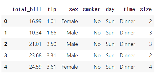
tips = sns.load_dataset('tips')
tips.head()

개요

• 파이썬에는 가상환경이 다양하게 존재한다.
• 이 중, conda와 virtualenv 가상환경에서 라이브러리 관리를 어떻게 하는지 비교를 해보도록 한다.

프로젝트 폴더 생성

• 폴더명은 virtualTest로 명명했다.

Conda

• 먼저 가상환경을 만들어본다.

conda create -n virtualTest python=3.10

• conda 가상환경에 접속하는 방법은 다음과 같다.

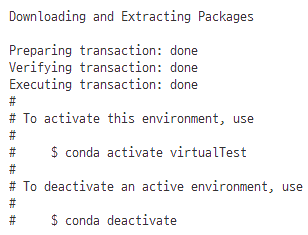
conda activate virtualTest

environment.yml

• 라이브러리 관리를 위해 아래와 같이 샘플 코드를 생성한다.

name: virtualTest
channels:
  - defaults
dependencies:
  - python=3.10
  - numpy
  - pandas
  - pip:
    - streamlit

• 실행 코드는 아래와 같다.

conda env create -f environment.yml

• 라이브러리 추가 설치를 한다.

conda install matplotlib

• 추가된 라이브러리를 추출한다.

conda env export > env_file.yml

• 파일을 확인하면 아래와 같이 복잡하게 나타난다.

개요

• 본 코드는 다음 유투브 영상에서 다룬 내용 중 다루지 못한 내용을 추가한 블로그입니다.

Youtube

• 유투브 영상은 다음과 같습니다. 전체 강의자료 및 데이터셋은 udemy 또는 inflern에서 확인 가능합니다.

가상의 데이터셋 생성

• 먼저 라이브러리를 불러온 후, 가상의 데이터셋을 만듭니다.

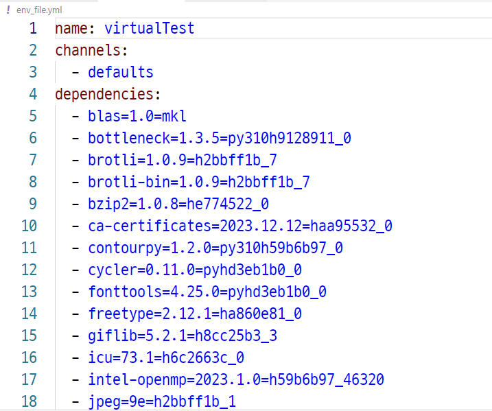
import matplotlib.pyplot as plt
import pandas as pd
import numpy as np

years = [2007, 2008]
months = ['1', '2', '3', '4', '5', '6', '7', '8', '9', '10', '11', '12']

np.random.seed(0)  # For reproducibility
data = {
    'year': np.repeat(years, 12),
    'month': months * 2,
    'house_prices': np.random.randint(100, 500, 24)
}

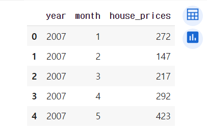
df_random = pd.DataFrame(data)

• 데이터셋은 크게 year, month, house_prices로 구성되어 있습니다.

df_random.head()

개요

• pandas 데이터프레임의 여러 개체 유형(문자열) 열에서 고유 값을 조사하려면 해당 열을 선택한 다음 unique()를 적용하여 고유 값을 추출한다. 이를 위한 단계별 접근 방식은 다음과 같다.
  • 1단계 : 여러 컬럼 중에서 문자열 컬럼만 추출한다.
  • 2단계 : unique() 함수를 활용하여 unique()값만 가져온다.
  • 3단계 : 결괏값은 dictionary 형태로 담는다.

가상 데이터 생성

• 임의의 가상 데이터를 생성한다.

import pandas as pd

data = {
    'Name': ['Evan', 'Bob', 'Evan', 'Bob'],
    'City': ['New York', 'Los Angeles', 'New York', 'SF'],
    'Job': ['Engineer', 'Engineer', 'Engineer', 'Artist'],
    'num1' : [1, 2, 3, 4]
}
df = pd.DataFrame(data)
print(df)

   Name         City       Job  num1
0  Evan     New York  Engineer     1
1   Bob  Los Angeles  Engineer     2
2  Evan     New York  Engineer     3
3   Bob           SF    Artist     4

object 컬럼 추출

# object 컬럼명 도출
object_cols = df.select_dtypes(include=['object'])
print(object_cols)

   Name         City       Job
0  Evan     New York  Engineer
1   Bob  Los Angeles  Engineer
2  Evan     New York  Engineer
3   Bob           SF    Artist

dictionary comprehension 활용한 고윳값 추출

• dictionary comprehension을 사용한다.
  • object_cols.columns는 고유값을 찾고자 하는 열들의 이름을 포함하는 리스트이다.
  • for col in object_cols.columns: 이 반복문은 object_cols.columns에 있는 각 열 이름에 대해 반복한다.
  • df[col].unique(): 이 부분은 DataFrame df에서 col 열의 고유값들을 추출합니다. unique() 함수는 해당 열에서 중복을 제거한 값들의 배열을 반환한다.
  • {col: df[col].unique() for …}: 이 구조는 각 열 이름(col)을 키로, 해당 열의 고유값 배열을 값으로 하는 딕셔너리를 생성한다.

# 각 컬럼별 고유값만 추출한다.
unique_values = {col: df[col].unique() for col in object_cols.columns}
unique_values

{'Name': array(['Evan', 'Bob'], dtype=object),
 'City': array(['New York', 'Los Angeles', 'SF'], dtype=object),
 'Job': array(['Engineer', 'Artist'], dtype=object)}

개요

• 작업 2유형(머신러닝)을 보다 쉽게 대비할 수 있도록 튜토리얼을 준비했습니다.
• 핵심 키워드 : Python 머신러닝은 pipeline 코드로 기억하자
• 본 코드는 구글 코랩에서 작성하였습니다.

유투브

• 유투브에서 강의 영상을 시청할 수 있습니다. (구독과 좋아요)

데이터 출처

• 본 데이터는 K-Data에서 가져왔습니다.

구글 드라이브 연동

• 데이터를 가져오기 위해 구글 드라이브와 연동합니다.

from google.colab import drive
drive.mount("/content/drive")

Mounted at /content/drive

라이브러리 불러오기

• 아래 라이브러리들을 모두 암기하시기를 바랍니다.

import pandas as pd
import numpy as np
from sklearn.model_selection import train_test_split
from sklearn.preprocessing import StandardScaler, OneHotEncoder
from sklearn.compose import ColumnTransformer
from sklearn.pipeline import Pipeline
## from sklearn.metrics import make_scorer, mean_squared_error
## from sklearn.ensemble import RandomForestRegressor

from sklearn.metrics import roc_auc_score
from sklearn.ensemble import RandomForestClassifier

데이터 가져오기

• 구글 드라이브에서 데이터를 가져옵니다.
• 시험장에서는 데이터 가져오기는 자동으로 설정이 되어 있습니다.

DATA_PATH = '/content/drive/MyDrive/Colab Notebooks/2024/빅분기/[Dataset] 작업형 제2유형/'

X_test = pd.read_csv(DATA_PATH + "X_test.csv", encoding='cp949')
X_train = pd.read_csv(DATA_PATH + "X_train.csv", encoding='cp949')
y_train = pd.read_csv(DATA_PATH + "y_train.csv", encoding='cp949')

print(X_test.shape, X_train.shape, y_train.shape)

(2482, 10) (3500, 10) (3500, 2)

데이터 정보 확인하기

• 분류 문제임을 확인할 수 있다.

print(y_train.head(3))

   cust_id  gender
0        0       0
1        1       0
2        2       1

• 문자열과 숫자 데이터가 적절하게 섞인 것을 확인할 수 있다.

print(X_train.head(3))

   cust_id      총구매액     최대구매액       환불금액   주구매상품 주구매지점  내점일수   내점당구매건수  \
0        0  68282840  11264000  6860000.0      기타   강남점    19  3.894737   
1        1   2136000   2136000   300000.0     스포츠   잠실점     2  1.500000   
2        2   3197000   1639000        NaN  남성 캐주얼   관악점     2  2.000000   

     주말방문비율  구매주기  
0  0.527027    17  
1  0.000000     1  
2  0.000000     1  

print(X_train.info())

<class 'pandas.core.frame.DataFrame'>
RangeIndex: 3500 entries, 0 to 3499
Data columns (total 10 columns):
 #   Column   Non-Null Count  Dtype  
---  ------   --------------  -----  
 0   cust_id  3500 non-null   int64  
 1   총구매액     3500 non-null   int64  
 2   최대구매액    3500 non-null   int64  
 3   환불금액     1205 non-null   float64
 4   주구매상품    3500 non-null   object 
 5   주구매지점    3500 non-null   object 
 6   내점일수     3500 non-null   int64  
 7   내점당구매건수  3500 non-null   float64
 8   주말방문비율   3500 non-null   float64
 9   구매주기     3500 non-null   int64  
dtypes: float64(3), int64(5), object(2)
memory usage: 273.6+ KB
None

print(y_train.info())

<class 'pandas.core.frame.DataFrame'>
RangeIndex: 3500 entries, 0 to 3499
Data columns (total 2 columns):
 #   Column   Non-Null Count  Dtype
---  ------   --------------  -----
 0   cust_id  3500 non-null   int64
 1   gender   3500 non-null   int64
dtypes: int64(2)
memory usage: 54.8 KB
None

데이터 전처리

• 2회-6회 시험까지 결측치는 존재하지 않았지만, 언제든지 결측치 처리 문제는 나올 수 있음.
• 결측치를 처리할 때는 fillna() 메서드를 사용한다.
  • 숫자는 각 컬럼의 평균대치, 문자는 최빈도값 대치를 한다.

X_train.isnull().sum()

cust_id       0
총구매액          0
최대구매액         0
환불금액       2295
주구매상품         0
주구매지점         0
내점일수          0
내점당구매건수       0
주말방문비율        0
구매주기          0
dtype: int64

• 여기에서는 특정 컬럼의 결측치가 많아서 삭제 한다.

X_train = X_train.drop("환불금액", axis=1)
X_train.isnull().sum()

cust_id    0
총구매액       0
최대구매액      0
주구매상품      0
주구매지점      0
내점일수       0
내점당구매건수    0
주말방문비율     0
구매주기       0
dtype: int64

X_train['주구매상품'].value_counts()

기타        595
가공식품      546
농산물       339
화장품       264
시티웨어      213
디자이너      193
수산품       153
캐주얼       101
명품        100
섬유잡화       98
골프         82
스포츠        69
일용잡화       64
모피/피혁      57
육류         57
남성 캐주얼     55
구두         54
건강식품       47
차/커피       44
피혁잡화       40
아동         40
축산가공       35
주방용품       32
셔츠         30
젓갈/반찬      29
주방가전       26
트래디셔널      23
남성정장       22
생활잡화       15
주류         14
가구         10
커리어         9
대형가전        8
란제리/내의      8
식기          7
액세서리        5
침구/수예       4
통신/컴퓨터      3
보석          3
남성 트랜디      2
소형가전        2
악기          2
Name: 주구매상품, dtype: int64

X_train['주구매지점'].value_counts()

본  점     1077
잠실점       474
분당점       436
부산본점      245
영등포점      241
일산점       198
강남점       145
광주점       114
노원점        90
청량리점       86
대전점        70
미아점        69
부평점        57
동래점        49
관악점        46
인천점        34
안양점        29
포항점        11
대구점         7
센텀시티점       6
울산점         6
전주점         5
창원점         4
상인점         1
Name: 주구매지점, dtype: int64

컬럼 분리

• cust_id는 별도로 분리한다.

X_train_id = X_train.pop("cust_id")
print(X_train.info())

<class 'pandas.core.frame.DataFrame'>
RangeIndex: 3500 entries, 0 to 3499
Data columns (total 8 columns):
 #   Column   Non-Null Count  Dtype  
---  ------   --------------  -----  
 0   총구매액     3500 non-null   int64  
 1   최대구매액    3500 non-null   int64  
 2   주구매상품    3500 non-null   object 
 3   주구매지점    3500 non-null   object 
 4   내점일수     3500 non-null   int64  
 5   내점당구매건수  3500 non-null   float64
 6   주말방문비율   3500 non-null   float64
 7   구매주기     3500 non-null   int64  
dtypes: float64(2), int64(4), object(2)
memory usage: 218.9+ KB
None

X_test_id = X_test.pop("cust_id")
print(X_test.info())

<class 'pandas.core.frame.DataFrame'>
RangeIndex: 2482 entries, 0 to 2481
Data columns (total 9 columns):
 #   Column   Non-Null Count  Dtype  
---  ------   --------------  -----  
 0   총구매액     2482 non-null   int64  
 1   최대구매액    2482 non-null   int64  
 2   환불금액     871 non-null    float64
 3   주구매상품    2482 non-null   object 
 4   주구매지점    2482 non-null   object 
 5   내점일수     2482 non-null   int64  
 6   내점당구매건수  2482 non-null   float64
 7   주말방문비율   2482 non-null   float64
 8   구매주기     2482 non-null   int64  
dtypes: float64(3), int64(4), object(2)
memory usage: 174.6+ KB
None

• 문자데이터와 숫자데이터 컬럼명만 추출한다.

cat_cols = X_train.select_dtypes(exclude = np.number).columns.tolist()
num_cols = X_train.select_dtypes(include = np.number).columns.tolist()
print(cat_cols)
print(num_cols)

['주구매상품', '주구매지점']
['총구매액', '최대구매액', '내점일수', '내점당구매건수', '주말방문비율', '구매주기']

데이터셋 분리

• 데이터셋 분리의 기본 원칙은 최대한 데이터의 분포가 일정해야 한다는 것이다.
• 평소 분석을 할 때는 하나씩 다 확인을 해야하지만, 시험장에서는 분류모델이 문제일 경우에는 y_train 데이터를 기준으로 층화추출을 한다.

X_tr, X_val, y_tr, y_val = train_test_split(
    X_train, y_train['gender'],
    stratify = y_train['gender'],
    test_size=0.3,
    random_state=42
)

X_tr.shape, X_val.shape, y_tr.shape, y_val.shape

((2450, 8), (1050, 8), (2450,), (1050,))

모델 만들기

모델 만들기 1 - 입문자

• 기본 모델만 만들고 싶다면 아래 코드만 기억한다.

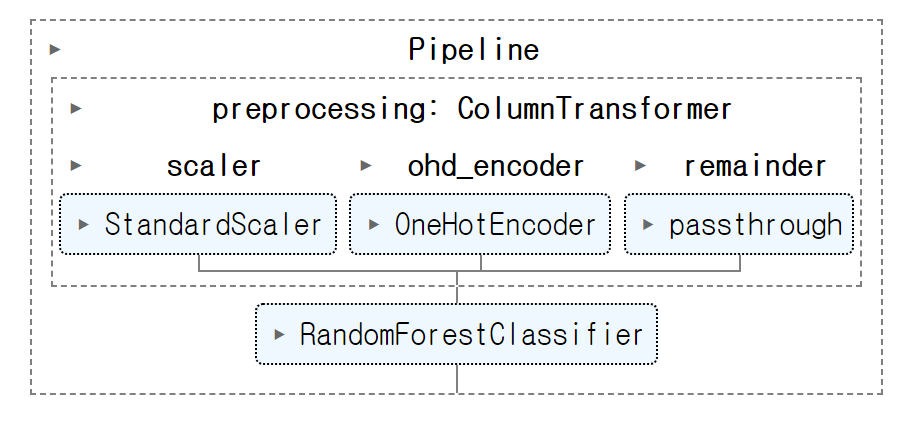
column_transformer = ColumnTransformer([
    ("scaler", StandardScaler(), num_cols),
    ("ohd_encoder", OneHotEncoder(handle_unknown='ignore'), cat_cols)
], remainder="passthrough")

pipeline = Pipeline([
    ("preprocessing", column_transformer),
    ("clf", RandomForestClassifier(random_state=42))
])

pipeline.fit(X_tr, y_tr)

개요

• Python 설치 과정을 유투브로 정리하였습니다.
• 본 튜토리얼은 Streamlit으로 프로젝트 한방에 끝내기 with 파이썬(2023, Sara & Evan) 교재를 동영상으로 변환하는 작업의 일환입니다.

유투브

개요

• BigQuery에서 Google Adwords 데이터와 Google Analytics를 불러올 수 있다.

전제조건

• 구글 클라우드 사용법은 어느정도 알고 있는 상태를 전제로 한다.
• Google Analytics를 이미 활용하고 있다는 것을 전제로 한다.

Google Analytics

• 왼쪽 메뉴에서 관리 > 제품 링크를 확인한다.

• BigQuery 링크 클릭 > 연결 버튼을 클릭한다.

• BigQuery 프로젝트를 선택한다.

• 활성화중인 프로젝트를 선택한다.

• 데이터 위치를 지정한다. 본 프로젝트에서는 서울로 명명한다.

• 내보내기 유형은 매일로 선택한다.

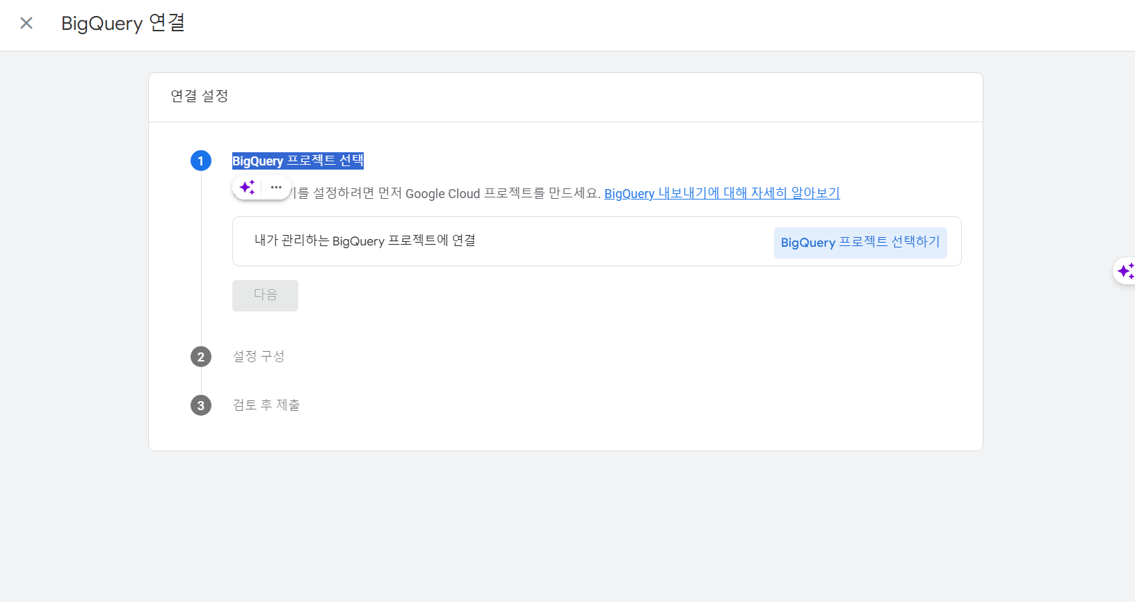
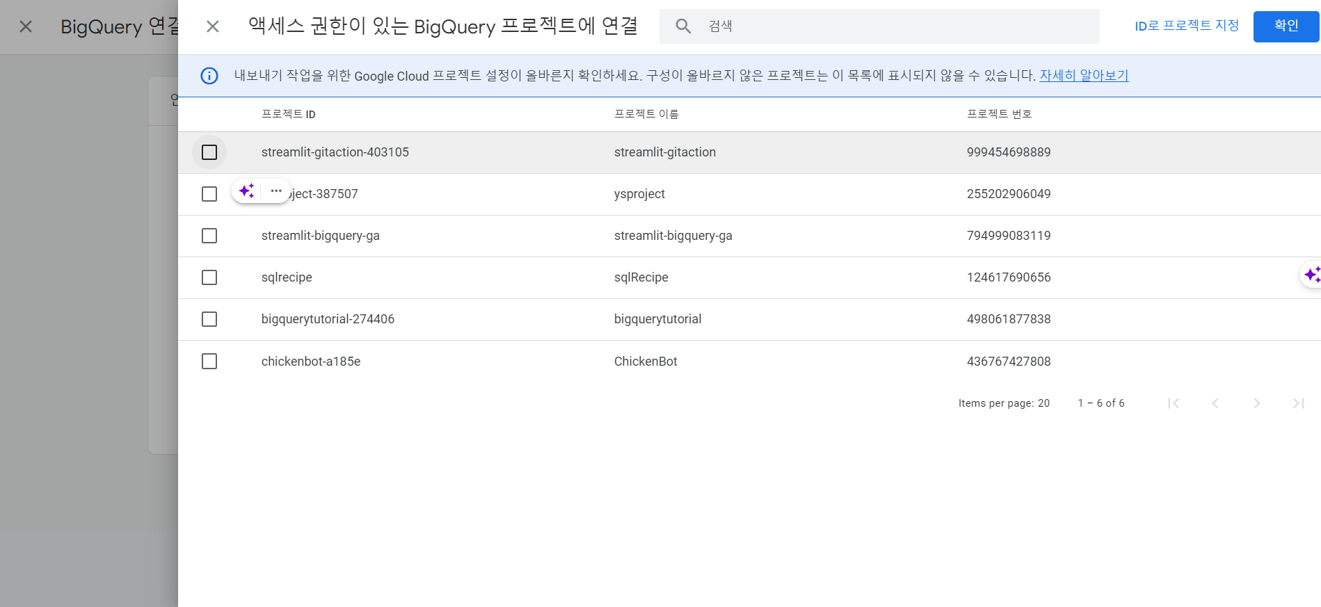
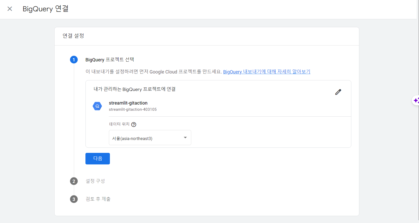
• 사용자 데이터는 일별로 선택한다.