머신러닝 알고리즘 - 결정트리 회귀모형

2020-09-03

Programming, Machine Learning, Python

Page content

I. 개요

결정트리 회귀 모형에 대해 배우도록 한다.
트리모형의 일반적인 특징에 대해 익힌다.

II. 결정 트리 모형

결정 트리는 분류, 회귀, 다중출력 작업도 가능한 활용범위가 많은 머신러닝 알고리즘이다.
결정 트리는 최근에 사용하는 랜덤포레스트, XGboost, LightGBM과 같은 모형의 기본 구성 요소이다.

(1) 의사결정 나무 예제

의사 결정 나무에서 자주 사용되는 예제를 우선 확인해보자.
먼저, 데이터셋을 기준으로 IRIS 붓꽃의 종류는 아래와 같이 3가지로 구성되어 있다.
- Versicolor, Setosa, Virginica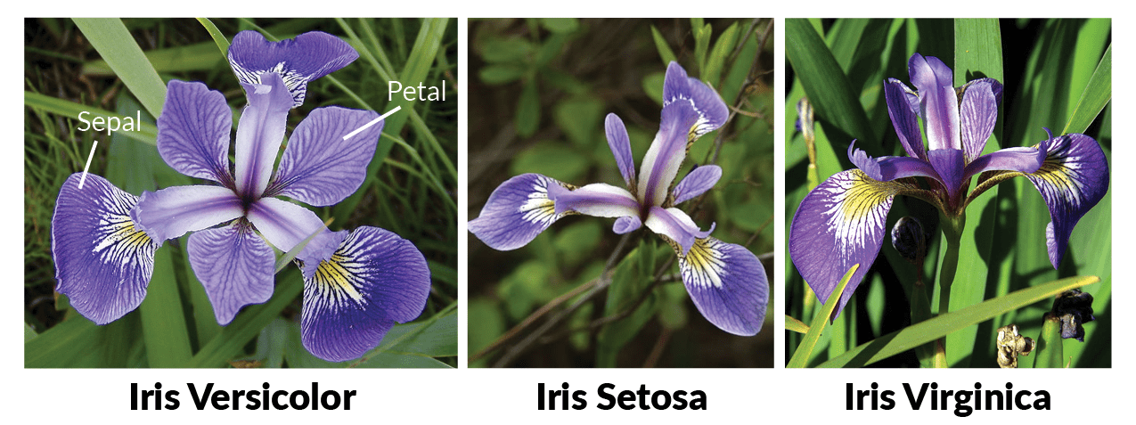
위 이미지에서 보는 것처럼, 종에 따라 잎의 크기가 다른 것을 확인할 수 있다. 이제 예제 데이터를 불러오는 것부터 시작해보자.

from sklearn.tree import DecisionTreeClassifier, plot_tree
from sklearn.datasets import load_iris
from sklearn.model_selection import train_test_split
import warnings
warnings.filterwarnings('ignore')

# 붓꽃 데이터를 로딩하고, 학습과 테스트 데이터 셋으로 분리
iris_data = load_iris()
X_train , X_test , y_train , y_test = train_test_split(iris_data.data, iris_data.target,
                                                       test_size=0.2,  random_state=11)

# DecisionTree Classifier 생성
dt_clf = DecisionTreeClassifier(random_state=156, max_depth = 2)


# DecisionTreeClassifer 학습. 
dt_clf.fit(X_train , y_train)

DecisionTreeClassifier(ccp_alpha=0.0, class_weight=None, criterion='gini',
                       max_depth=2, max_features=None, max_leaf_nodes=None,
                       min_impurity_decrease=0.0, min_impurity_split=None,
                       min_samples_leaf=1, min_samples_split=2,
                       min_weight_fraction_leaf=0.0, presort='deprecated',
                       random_state=156, splitter='best')

import matplotlib.pyplot as plt

explt_vars = ["sepal_length", "sepal_width", "petal_length", "petal_width"]
fct_val = {0: 'setosa', 1: 'versicolor', 2: "virginica"}

plt.figure(figsize = (10,8))
plot_tree(dt_clf, feature_names = explt_vars, class_names = fct_val, filled = True);

png

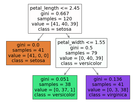
우선 의사결정 나무의 큰 특징은 매우 직관적이다. 먼저 뿌리노드 (깊이가 0인 맨 꼭대기의 노드)에서 시작한다.
- petal_length의 2.45cm 보다 짧은지 검사하여 True인 경우는 왼쪽으로 False인 경우는 오른쪽으로 1차적으로 분류한다.
- 이 때, 리프 노드는 분류의 마지막 지점이기 때문에 더 이상 추가적인 검사를 하지 않는다.
결정트리의 결과값 해석은 이게 끝이다.
또 하나의 특징은, 일반적인 선형회귀와 다르게 데이터 전처리가 거의 필요하지 않다.

(2) 불순도

지니 불순도의 개념
- 한 노드의 모든 샘플이 같은 클래스에 속해 있다면 이 노드를 순수(gini=0)이라고 함 $$G_{i} = 1 - \sum_{k=1}^{n}\left ( P_{i,k} \right )^{2}$$
위 gini=0.136 나온 것을 확인하면 다음과 같다.

gini = 1 - (0/41)**2 - (3/41)**2 - (38/41)**2
print('The value of Gini is: {:.3f}'.format(gini))

The value of Gini is: 0.136

(3) 결정 트리의 경계

결정 트리의 결정 경계를 보여주는 시각화를 작성한다.
소스코드 출처(핸즈온 머신러닝 2)

from matplotlib.colors import ListedColormap
from sklearn.datasets import load_iris
from sklearn.tree import DecisionTreeClassifier
import numpy as np

iris = load_iris()
X = iris.data[:, 2:] # 꽃잎 길이와 너비
y = iris.target

tree_clf = DecisionTreeClassifier(max_depth=2, random_state=42)
tree_clf.fit(X, y)

def plot_decision_boundary(clf, X, y, axes=[0, 7.5, 0, 3], iris=True, legend=False, plot_training=True):
    x1s = np.linspace(axes[0], axes[1], 100)
    x2s = np.linspace(axes[2], axes[3], 100)
    x1, x2 = np.meshgrid(x1s, x2s)
    X_new = np.c_[x1.ravel(), x2.ravel()]
    y_pred = clf.predict(X_new).reshape(x1.shape)
    custom_cmap = ListedColormap(['#fafab0','#9898ff','#a0faa0'])
    plt.contourf(x1, x2, y_pred, alpha=0.3, cmap=custom_cmap)
    if not iris:
        custom_cmap2 = ListedColormap(['#7d7d58','#4c4c7f','#507d50'])
        plt.contour(x1, x2, y_pred, cmap=custom_cmap2, alpha=0.8)
    if plot_training:
        plt.plot(X[:, 0][y==0], X[:, 1][y==0], "yo", label="Iris setosa")
        plt.plot(X[:, 0][y==1], X[:, 1][y==1], "bs", label="Iris versicolor")
        plt.plot(X[:, 0][y==2], X[:, 1][y==2], "g^", label="Iris virginica")
        plt.axis(axes)
    if iris:
        plt.xlabel("Petal length", fontsize=14)
        plt.ylabel("Petal width", fontsize=14)
    else:
        plt.xlabel(r"$x_1$", fontsize=18)
        plt.ylabel(r"$x_2$", fontsize=18, rotation=0)
    if legend:
        plt.legend(loc="lower right", fontsize=14)

plt.figure(figsize=(8, 4))
plot_decision_boundary(tree_clf, X, y)
plt.plot([2.45, 2.45], [0, 3], "k-", linewidth=2)
plt.plot([2.45, 7.5], [1.75, 1.75], "k--", linewidth=2)
plt.plot([4.95, 4.95], [0, 1.75], "k:", linewidth=2)
plt.plot([4.85, 4.85], [1.75, 3], "k:", linewidth=2)
plt.text(1.40, 1.0, "Depth=0", fontsize=15)
plt.text(3.2, 1.80, "Depth=1", fontsize=13)
plt.text(4.05, 0.5, "(Depth=2)", fontsize=11)

Text(4.05, 0.5, '(Depth=2)')

png

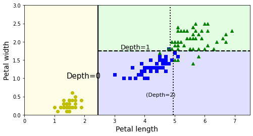
Depth = 0: Petal_Length의 길이 2.45cm를 의미한다.
Depth = 1: Petal_Length이 길이 1.55cm를 의미한다.

(4) 규제 매개변수

기본 개념: 훈련 데이터에 대한 과대적합을 피하기 위해 학습할 때, 결정 트리의 자유도를 제한한다.
기본값에서 None의 의미는 제한이 없음을 의미한다.
- 즉, 과적합이 되기 싶다는 뜻이다.
규제 매개변수에 관한 대략적인 설명은 다음과 같다.
- min_samples_split: 분할되기 위해 노드가 가져야 최소 샘플 수
- min_samples_leaf: 리프 노드가 가지고 있어야 할 최소 샘플 수
- min_weight_fraction_leaf: 가중치가 부여된 전체 샘플 수에서의 비율
- max_leaf_nodes: 리프 노드의 최대 수
- max_features: 각 노드에서 분할에 사용할 특성의 최대 수
min_으로 시작하는 것을 증가시키거나, 도는 max_으로 시작하는 것을 감소시키면 모델에 규제가 커짐.
- pruning: 가지치기의 일종으로 순도를 높이는 것이 통계적으로 효과가 없다면 리프 노드 바로 위의 노드는 불필요하다. (이 때, 카이제곱 검정을 사용함).

III. 결정 트리 회귀 모형 예제

이러한 사전 지식을 배경으로 회귀 모형을 만듭니다.

(1) 데이터셋 만들기

지난 선형회귀 때와 동일한 데이터를 학습합니다.

from sklearn.model_selection import train_test_split
from sklearn.tree import DecisionTreeRegressor
from sklearn.metrics import mean_squared_error, r2_score
import pandas as pd
from sklearn.datasets import load_boston

boston_raw = load_boston()
def sklearn_to_df(sklearn_dataset):
    df = pd.DataFrame(sklearn_dataset.data, columns=sklearn_dataset.feature_names)
    df['target'] = pd.Series(sklearn_dataset.target)
    return df

df_boston = sklearn_to_df(boston_raw)
df_boston = df_boston.rename({"target": "MEDV"}, axis='columns')

# 종속변수 및 독립변수 데이터 셋으로 분리
y_target = df_boston['MEDV']
X_data = df_boston.drop(['MEDV'], axis = 1, inplace=False)

X_train, X_test, y_train, y_test = train_test_split(X_data, y_target, test_size=0.3, random_state=1)
X_train.shape, X_test.shape, y_train.shape, y_test.shape

((354, 13), (152, 13), (354,), (152,))

(2) 결정 트리 모형 만들기

간단하게 코드를 구현해보자.

my_1st_tree = DecisionTreeRegressor(max_depth=5, random_state=42)
my_1st_tree.fit(X_train, y_train)

DecisionTreeRegressor(ccp_alpha=0.0, criterion='mse', max_depth=5,
                      max_features=None, max_leaf_nodes=None,
                      min_impurity_decrease=0.0, min_impurity_split=None,
                      min_samples_leaf=1, min_samples_split=2,
                      min_weight_fraction_leaf=0.0, presort='deprecated',
                      random_state=42, splitter='best')

(3) 모형 예측 및 평가

적합된 모형을 예측하고 평가하도록 한다.

y_preds = my_1st_tree.predict(X_test)
mse = mean_squared_error(y_test, y_preds)
rmse = np.sqrt(mse)
r2_points = r2_score(y_test, y_preds)
print("RMSE:", rmse)
print("R^2:", r2_points)

RMSE: 3.738238738077283
R^2: 0.8475314269410481

지난 선형 회귀 때와 비교하면 다음과 같이 정리할 수 있다.

모델	RMSE	R2score
선형회귀	4.45	0.78
결정트리회귀(max_depth=2)	5.06	0.72
결정트리회귀(max_depth=3)	4.21	0.80
결정트리회귀(max_depth=4)	3.52	0.86
결정트리회귀(max_depth=5)	3.73	0.84

max_depth의 옵션을 변동하면, RMSE와 $R^2$ 점수가 변동되는 것을 확인할 수 있다.

IV. 결론

이제 모형을 2개 배웠다.
- 선형회귀와, 트리모형, 모형은 매우 많기 때문에 일일이 다 알려드리는 것은 매우 비효율적이다.
- 그럼 각각 일일이 다 공부하는 게 의미가 있는 것인가?
- 모든 통계 모형을 한꺼번에 다 공부하는 것은 지양한다.
  - 시간이 해결해준다. 그리고, 최신 논문을 늘 챙긴다.
- 이제 나무 모형으로 넘어간다. 현재 나오는 최신 알고리즘은 나무 모형에 기반하기 때문이다.
이 때, 우리가 기억해야 하는 것은 모형의 평가다.
- 예측에서 중요한 것은 예측값과 실제값의 오차를 줄이는 것. 이것만 기억하자.
- 모형의 원리를 깊이 몰라도, 예측 지표에 대한 평가는 할 수 있다.
- RMSE와 $R^2$를 기억해야 한다.
이제 본격적으로 캐글 데이터를 만져본다.
- 지금까지는 깔끔한(Clean) 데이터를 가지고 했다.
- 실무는 배우 지저분하다.