삼성카드 대회 Track-2 - 포지셔닝 분석(2)

대회 소개

  • 삼성카드 데이터분석 공모전이 시행되고 있다.
    • 대회에 처음 참여하는 아시아경제-수강생들을 위해 일종의 가이드라인으로 제안하고자 한다.
  • 본 포스트에서는 기본적인 내용만 전달하고자 함을 밝힌다.
    • Track2 과정은 마케팅 전략 제안이 중요하다!

포지셔닝 분석 개요

  • 마케팅에서 자주 보는 분석 방법중의 하나는 포지셔닝(Positioning) 기법이다.
  • 포지셔닝 분석은 마케팅 통계분석 기법중의 하나로, 기업이나, 상품, 브랜드 같은 개체들의 포지셔닝을 수행하는 다차원 척도법(MDS: Multi-Dimensional Scaling)과 상응분석(Correspondence Analysis)이 있다.
  • 위 두가지 분석 방법 중 무엇을 사용해야 할까?
    • 만약 데이터셋이 주로 등간척도, 비율척도와 같이 구성되어 있다면 다차원 척도법
    • 만약 데이터셋이 주로 명목척도, 서열척도와 같이 구성되어 있다면 상응분석
  • 현재 삼성카드 대회의 주 데이터셋은 명목척도 및 서열척도로 구성되어 있기 때문에 상응분석으로 시작하면 된다.

상응분석

(1) 기본 개념

  • 상응분석을 사용하려면 빈도교차표를 만들어야 한다.
  • 요약하면, 상응분석은 범주형 변수의 빈도를 나타내고 있는 빈도교차표의 행과 열(명목변수의 범주 값들)을 그래프상의 자극점 형태로 표시하는 방법.
  • 이 때, 단순 상응분석은 2개의 변수, 다중 상응분석은 3개 이상의 변수 활용한다.
  • 이 때, 상응분석은 카이제곱 검정과 같이 범주형 변수간의 상호연관성을 바탕으로 진행된다.
    • 따라서, 두 개의 범주형 변수가 서로 연관성을 가지고 있다는 전제하에서 진행된다.

(2) 데이터 불러오기

  • 먼저 필요한 데이터를 불러온다.
  • 필자는 구글 코랩에서 데이터를 불러오기 때문에
%config InlineBackend.figure_format = 'retina'
!sudo apt-get -qq -y install fonts-nanum
The following package was automatically installed and is no longer required:
  libnvidia-common-440
Use 'apt autoremove' to remove it.
The following NEW packages will be installed:
  fonts-nanum
0 upgraded, 1 newly installed, 0 to remove and 39 not upgraded.
Need to get 9,604 kB of archives.
After this operation, 29.5 MB of additional disk space will be used.
Selecting previously unselected package fonts-nanum.
(Reading database ... 144579 files and directories currently installed.)
Preparing to unpack .../fonts-nanum_20170925-1_all.deb ...
Unpacking fonts-nanum (20170925-1) ...
Setting up fonts-nanum (20170925-1) ...
Processing triggers for fontconfig (2.12.6-0ubuntu2) ...
import seaborn as sns
import pandas as pd
import matplotlib.pyplot as plt
import matplotlib as mpl
import matplotlib.font_manager as fm
/usr/local/lib/python3.6/dist-packages/statsmodels/tools/_testing.py:19: FutureWarning: pandas.util.testing is deprecated. Use the functions in the public API at pandas.testing instead.
  import pandas.util.testing as tm
for font in fm.fontManager.ttflist:
    if 'Nanum' in font.name:
        print(font.name, font.fname)
NanumGothic /usr/share/fonts/truetype/nanum/NanumGothic.ttf
NanumSquareRound /usr/share/fonts/truetype/nanum/NanumSquareRoundR.ttf
NanumSquare /usr/share/fonts/truetype/nanum/NanumSquareR.ttf
NanumSquareRound /usr/share/fonts/truetype/nanum/NanumSquareRoundB.ttf
NanumBarunGothic /usr/share/fonts/truetype/nanum/NanumBarunGothicBold.ttf
NanumMyeongjo /usr/share/fonts/truetype/nanum/NanumMyeongjo.ttf
NanumMyeongjo /usr/share/fonts/truetype/nanum/NanumMyeongjoBold.ttf
NanumBarunGothic /usr/share/fonts/truetype/nanum/NanumBarunGothic.ttf
NanumSquare /usr/share/fonts/truetype/nanum/NanumSquareB.ttf
NanumGothic /usr/share/fonts/truetype/nanum/NanumGothicBold.ttf
fontpath = '/usr/share/fonts/truetype/nanum/NanumGothic.ttf'
font = fm.FontProperties(fname=fontpath, size=9)
plt.rc('font', family='NanumGothic') 
plt.rcParams["figure.figsize"] = (20, 10)
plt.rcParams['lines.linewidth'] = 2
plt.rcParams['lines.color'] = 'r'
plt.rcParams['axes.grid'] = True 
mpl.font_manager._rebuild()
fm._rebuild()
  • 한글 텍스트가 잘 나오는지 확인해본다.
font = {'family' : 'NanumGothic',
        'weight' : 'bold',
        'size'   : 22}

plt.rc('font', **font)
plt.text(0.3, 0.3, '한글', size=100)
Text(0.3, 0.3, '한글')

png

삼성카드 대회 Track-2 - 포지셔닝 분석(1)

대회 소개

  • 삼성카드 데이터분석 공모전이 시행되고 있다.
    • 대회에 처음 참여하는 아시아경제-수강생들을 위해 일종의 가이드라인으로 제안하고자 한다.
  • 본 포스트에서는 기본적인 내용만 전달하고자 함을 밝힌다.
    • Track2 과정은 마케팅 전략 제안이 중요하다!

포지셔닝 분석 개요

  • 마케팅에서 자주 보는 분석 방법중의 하나는 포지셔닝(Positioning) 기법이다.
  • 포지셔닝 분석은 마케팅 통계분석 기법중의 하나로, 기업이나, 상품, 브랜드 같은 개체들의 포지셔닝을 수행하는 다차원 척도법(MDS: Multi-Dimensional Scaling)과 상응분석(Correspondence Analysis)이 있다.
  • 위 두가지 분석 방법 중 무엇을 사용해야 할까?
    • 만약 데이터셋이 주로 등간척도, 비율척도와 같이 구성되어 있다면 다차원 척도법
    • 만약 데이터셋이 주로 명목척도, 서열척도와 같이 구성되어 있다면 상응분석
  • 현재 삼성카드 대회의 주 데이터셋은 명목척도 및 서열척도로 구성되어 있기 때문에 상응분석으로 시작하면 된다.

상응분석

  • Correspondence Analysis는 범주형 변수(수준)들 간의 연관성을 분석한 후, 그 결과를 시각적 해석이 용이하도록 그래프화 하는 것임

(1) 기본 개념

  • 상응분석을 사용하려면 빈도교차표를 만들어야 한다.
  • 요약하면, 상응분석은 범주형 변수의 빈도를 나타내고 있는 빈도교차표의 행과 열(명목변수의 범주 값들)을 그래프상의 자극점 형태로 표시하는 방법.
  • 이 때, 단순 상응분석은 2개의 변수, 다중 상응분석은 3개 이상의 변수 활용한다.
  • 이 때, 상응분석은 카이제곱 검정과 같이 범주형 변수간의 상호연관성을 바탕으로 진행된다.
    • 따라서, 두 개의 범주형 변수가 서로 연관성을 가지고 있다는 전제하에서 진행된다.

(2) 데이터 불러오기

  • 먼저 필요한 데이터를 불러온다.
  • 필자는 구글 코랩에서 데이터를 불러오기 때문에
%config InlineBackend.figure_format = 'retina'
!sudo apt-get -qq -y install fonts-nanum
The following package was automatically installed and is no longer required:
  libnvidia-common-440
Use 'apt autoremove' to remove it.
The following NEW packages will be installed:
  fonts-nanum
0 upgraded, 1 newly installed, 0 to remove and 39 not upgraded.
Need to get 9,604 kB of archives.
After this operation, 29.5 MB of additional disk space will be used.
Selecting previously unselected package fonts-nanum.
(Reading database ... 144579 files and directories currently installed.)
Preparing to unpack .../fonts-nanum_20170925-1_all.deb ...
Unpacking fonts-nanum (20170925-1) ...
Setting up fonts-nanum (20170925-1) ...
Processing triggers for fontconfig (2.12.6-0ubuntu2) ...
import seaborn as sns
import pandas as pd
import matplotlib.pyplot as plt
import matplotlib as mpl
import matplotlib.font_manager as fm
/usr/local/lib/python3.6/dist-packages/statsmodels/tools/_testing.py:19: FutureWarning: pandas.util.testing is deprecated. Use the functions in the public API at pandas.testing instead.
  import pandas.util.testing as tm
for font in fm.fontManager.ttflist:
    if 'Nanum' in font.name:
        print(font.name, font.fname)
NanumGothic /usr/share/fonts/truetype/nanum/NanumGothicBold.ttf
NanumBarunGothic /usr/share/fonts/truetype/nanum/NanumBarunGothic.ttf
NanumBarunGothic /usr/share/fonts/truetype/nanum/NanumBarunGothicBold.ttf
NanumSquare /usr/share/fonts/truetype/nanum/NanumSquareB.ttf
NanumMyeongjo /usr/share/fonts/truetype/nanum/NanumMyeongjoBold.ttf
NanumSquareRound /usr/share/fonts/truetype/nanum/NanumSquareRoundB.ttf
NanumSquare /usr/share/fonts/truetype/nanum/NanumSquareR.ttf
NanumMyeongjo /usr/share/fonts/truetype/nanum/NanumMyeongjo.ttf
NanumSquareRound /usr/share/fonts/truetype/nanum/NanumSquareRoundR.ttf
NanumGothic /usr/share/fonts/truetype/nanum/NanumGothic.ttf
fontpath = '/usr/share/fonts/truetype/nanum/NanumGothic.ttf'
font = fm.FontProperties(fname=fontpath, size=9)
plt.rc('font', family='NanumGothic') 
plt.rcParams["figure.figsize"] = (20, 10)
plt.rcParams['lines.linewidth'] = 2
plt.rcParams['lines.color'] = 'r'
plt.rcParams['axes.grid'] = True 
mpl.font_manager._rebuild()
fm._rebuild()
  • 한글 텍스트가 잘 나오는지 확인해본다.
font = {'family' : 'NanumGothic',
        'weight' : 'bold',
        'size'   : 22}

plt.rc('font', **font)
plt.text(0.3, 0.3, '한글', size=100)
Text(0.3, 0.3, '한글')

png

머신러닝 알고리즘 - 결정트리 회귀모형

I. 개요

  • 결정트리 회귀 모형에 대해 배우도록 한다.
  • 트리모형의 일반적인 특징에 대해 익힌다.

II. 결정 트리 모형

  • 결정 트리는 분류, 회귀, 다중출력 작업도 가능한 활용범위가 많은 머신러닝 알고리즘이다.
  • 결정 트리는 최근에 사용하는 랜덤포레스트, XGboost, LightGBM과 같은 모형의 기본 구성 요소이다.

(1) 의사결정 나무 예제

  • 의사 결정 나무에서 자주 사용되는 예제를 우선 확인해보자.

  • 먼저, 데이터셋을 기준으로 IRIS 붓꽃의 종류는 아래와 같이 3가지로 구성되어 있다.

    • Versicolor, Setosa, Virginica
  • 위 이미지에서 보는 것처럼, 종에 따라 잎의 크기가 다른 것을 확인할 수 있다. 이제 예제 데이터를 불러오는 것부터 시작해보자.

Python 통계 - 포지셔닝 분석(2)

강의 홍보

포지셔닝 분석 개요

  • 마케팅에서 자주 보는 분석 방법중의 하나는 포지셔닝(Positioning) 기법이다.
  • 포지셔닝 분석은 마케팅 통계분석 기법중의 하나로, 기업이나, 상품, 브랜드 같은 개체들의 포지셔닝을 수행하는 다차원 척도법(MDS: Multi-Dimensional Scaling)과 상응분석(Correspondence Analysis)이 있다.
  • 위 두가지 분석 방법 중 무엇을 사용해야 할까?
    • 만약 데이터셋이 주로 등간척도, 비율척도와 같이 구성되어 있다면 다차원 척도법
    • 만약 데이터셋이 주로 명목척도, 서열척도와 같이 구성되어 있다면 상응분석
  • 현재 삼성카드 대회의 주 데이터셋은 명목척도 및 서열척도로 구성되어 있기 때문에 상응분석으로 시작하면 된다.

상응분석

  • Correspondence Analysis는 범주형 변수(수준)들 간의 연관성을 분석한 후, 그 결과를 시각적 해석이 용이하도록 그래프화 하는 것임

(1) 기본 개념

  • 상응분석을 사용하려면 빈도교차표를 만들어야 한다.
  • 요약하면, 상응분석은 범주형 변수의 빈도를 나타내고 있는 빈도교차표의 행과 열(명목변수의 범주 값들)을 그래프상의 자극점 형태로 표시하는 방법.
  • 이 때, 단순 상응분석은 2개의 변수, 다중 상응분석은 3개 이상의 변수 활용한다.
  • 이 때, 상응분석은 카이제곱 검정과 같이 범주형 변수간의 상호연관성을 바탕으로 진행된다.
    • 따라서, 두 개의 범주형 변수가 서로 연관성을 가지고 있다는 전제하에서 진행된다.

(2) 데이터 불러오기

  • 먼저 필요한 데이터를 불러온다.
  • 필자는 구글 코랩에서 데이터를 불러오기 때문에
%config InlineBackend.figure_format = 'retina'
!apt -qq -y install fonts-nanum
fonts-nanum is already the newest version (20170925-1).
The following package was automatically installed and is no longer required:
  libnvidia-common-440
Use 'apt autoremove' to remove it.
0 upgraded, 0 newly installed, 0 to remove and 39 not upgraded.
import seaborn as sns
import pandas as pd
import matplotlib.pyplot as plt
import matplotlib as mpl
import matplotlib.font_manager as fm
/usr/local/lib/python3.6/dist-packages/statsmodels/tools/_testing.py:19: FutureWarning: pandas.util.testing is deprecated. Use the functions in the public API at pandas.testing instead.
  import pandas.util.testing as tm
for font in fm.fontManager.ttflist:
    if 'Nanum' in font.name:
        print(font.name, font.fname)
NanumMyeongjo /usr/share/fonts/truetype/nanum/NanumMyeongjo.ttf
NanumSquare /usr/share/fonts/truetype/nanum/NanumSquareR.ttf
NanumSquare /usr/share/fonts/truetype/nanum/NanumSquareB.ttf
NanumBarunGothic /usr/share/fonts/truetype/nanum/NanumBarunGothicBold.ttf
NanumMyeongjo /usr/share/fonts/truetype/nanum/NanumMyeongjoBold.ttf
NanumSquareRound /usr/share/fonts/truetype/nanum/NanumSquareRoundR.ttf
NanumSquareRound /usr/share/fonts/truetype/nanum/NanumSquareRoundB.ttf
NanumBarunGothic /usr/share/fonts/truetype/nanum/NanumBarunGothic.ttf
NanumGothic /usr/share/fonts/truetype/nanum/NanumGothic.ttf
NanumGothic /usr/share/fonts/truetype/nanum/NanumGothicBold.ttf
fontpath = '/usr/share/fonts/truetype/nanum/NanumGothic.ttf'
font = fm.FontProperties(fname=fontpath, size=9)
plt.rc('font', family='NanumGothic') 
plt.rcParams["figure.figsize"] = (20, 10)
plt.rcParams['lines.linewidth'] = 2
plt.rcParams['lines.color'] = 'r'
plt.rcParams['axes.grid'] = True 
mpl.font_manager._rebuild()
fm._rebuild()
font = {'family' : 'NanumGothic',
        'weight' : 'bold',
        'size'   : 22}

plt.rc('font', **font)
plt.text(0.3, 0.3, '한글', size=100)
Text(0.3, 0.3, '한글')

png

Python 통계 - 포지셔닝 분석(1)

강의 홍보

포지셔닝 분석 개요

  • 마케팅에서 자주 보는 분석 방법중의 하나는 포지셔닝(Positioning) 기법이다.
  • 포지셔닝 분석은 마케팅 통계분석 기법중의 하나로, 기업이나, 상품, 브랜드 같은 개체들의 포지셔닝을 수행하는 다차원 척도법(MDS: Multi-Dimensional Scaling)과 상응분석(Correspondence Analysis)이 있다.
  • 위 두가지 분석 방법 중 무엇을 사용해야 할까?
    • 만약 데이터셋이 주로 등간척도, 비율척도와 같이 구성되어 있다면 다차원 척도법
    • 만약 데이터셋이 주로 명목척도, 서열척도와 같이 구성되어 있다면 상응분석
  • 현재 삼성카드 대회의 주 데이터셋은 명목척도 및 서열척도로 구성되어 있기 때문에 상응분석으로 시작하면 된다.

상응분석

  • Correspondence Analysis는 범주형 변수(수준)들 간의 연관성을 분석한 후, 그 결과를 시각적 해석이 용이하도록 그래프화 하는 것임

(1) 기본 개념

  • 상응분석을 사용하려면 빈도교차표를 만들어야 한다.
  • 요약하면, 상응분석은 범주형 변수의 빈도를 나타내고 있는 빈도교차표의 행과 열(명목변수의 범주 값들)을 그래프상의 자극점 형태로 표시하는 방법.
  • 이 때, 단순 상응분석은 2개의 변수, 다중 상응분석은 3개 이상의 변수 활용한다.
  • 이 때, 상응분석은 카이제곱 검정과 같이 범주형 변수간의 상호연관성을 바탕으로 진행된다.
    • 따라서, 두 개의 범주형 변수가 서로 연관성을 가지고 있다는 전제하에서 진행된다.

(2) 데이터 불러오기

  • 먼저 필요한 데이터를 불러온다.
  • 필자는 구글 코랩에서 데이터를 불러오기 때문에
%config InlineBackend.figure_format = 'retina'
!apt -qq -y install fonts-nanum
fonts-nanum is already the newest version (20170925-1).
The following package was automatically installed and is no longer required:
  libnvidia-common-440
Use 'apt autoremove' to remove it.
0 upgraded, 0 newly installed, 0 to remove and 39 not upgraded.
import seaborn as sns
import pandas as pd
import matplotlib.pyplot as plt
import matplotlib as mpl
import matplotlib.font_manager as fm
/usr/local/lib/python3.6/dist-packages/statsmodels/tools/_testing.py:19: FutureWarning: pandas.util.testing is deprecated. Use the functions in the public API at pandas.testing instead.
  import pandas.util.testing as tm
for font in fm.fontManager.ttflist:
    if 'Nanum' in font.name:
        print(font.name, font.fname)
NanumMyeongjo /usr/share/fonts/truetype/nanum/NanumMyeongjoBold.ttf
NanumSquareRound /usr/share/fonts/truetype/nanum/NanumSquareRoundR.ttf
NanumSquare /usr/share/fonts/truetype/nanum/NanumSquareB.ttf
NanumGothic /usr/share/fonts/truetype/nanum/NanumGothicBold.ttf
NanumMyeongjo /usr/share/fonts/truetype/nanum/NanumMyeongjo.ttf
NanumGothic /usr/share/fonts/truetype/nanum/NanumGothic.ttf
NanumBarunGothic /usr/share/fonts/truetype/nanum/NanumBarunGothicBold.ttf
NanumSquareRound /usr/share/fonts/truetype/nanum/NanumSquareRoundB.ttf
NanumBarunGothic /usr/share/fonts/truetype/nanum/NanumBarunGothic.ttf
NanumSquare /usr/share/fonts/truetype/nanum/NanumSquareR.ttf
fontpath = '/usr/share/fonts/truetype/nanum/NanumGothic.ttf'
font = fm.FontProperties(fname=fontpath, size=9)
plt.rc('font', family='NanumGothic') 
plt.rcParams["figure.figsize"] = (20, 10)
plt.rcParams['lines.linewidth'] = 2
plt.rcParams['lines.color'] = 'r'
plt.rcParams['axes.grid'] = True 
mpl.font_manager._rebuild()
fm._rebuild()
font = {'family' : 'NanumGothic',
        'weight' : 'bold',
        'size'   : 22}

plt.rc('font', **font)
plt.text(0.3, 0.3, '한글', size=100)
Text(0.3, 0.3, '한글')

png

삼성카드 대회 Track-2 - matplotlib 막대 그래프

대회 소개

  • 삼성카드 데이터분석 공모전이 시행되고 있다.
    • 대회에 처음 참여하는 아시아경제-수강생들을 위해 일종의 가이드라인으로 제안하고자 한다.
  • 본 포스트에서는 기본적인 내용만 전달하고자 함을 밝힌다.
    • Track2 과정은 마케팅 전략 제안이 중요하다!

환경 세팅

  • 먼저, 데이터가 모두 한글로 구성이 되어 있기 때문에 한글파일 설정부터 진행한다.
  • 한글파일 설정이 완료되면 구글 드라이브와 연동한다.
  • 데이터 시각화를 진행한다.
%config InlineBackend.figure_format = 'retina'
!sudo apt-get -qq -y install fonts-nanum
fonts-nanum is already the newest version (20170925-1).
The following package was automatically installed and is no longer required:
  libnvidia-common-440
Use 'apt autoremove' to remove it.
0 upgraded, 0 newly installed, 0 to remove and 39 not upgraded.
import seaborn as sns
import pandas as pd
import matplotlib.pyplot as plt
import matplotlib as mpl
import matplotlib.font_manager as fm
/usr/local/lib/python3.6/dist-packages/statsmodels/tools/_testing.py:19: FutureWarning: pandas.util.testing is deprecated. Use the functions in the public API at pandas.testing instead.
  import pandas.util.testing as tm
fontpath = '/usr/share/fonts/truetype/nanum/NanumBarunGothic.ttf'
font = fm.FontProperties(fname=fontpath, size=9)
plt.rc('font', family='NanumBarunGothic') 
plt.rcParams["figure.figsize"] = (20, 10)
mpl.font_manager._rebuild()
mpl.pyplot.rc('font', family='NanumGothic')
fm._rebuild()
  • 여기까지 실행하였으면 구글 코랩에서 런타임-런타임 다시 시작을 클릭한다.

구글 드라이브 연동

  • 이제 구글 드라이브를 연동한다.
# Mount Google Drive
from google.colab import drive # import drive from google colab

ROOT = "/content/drive"     # default location for the drive
print(ROOT)                 # print content of ROOT (Optional)
drive.mount(ROOT)           # we mount the google drive at /content/drive
/content/drive
Drive already mounted at /content/drive; to attempt to forcibly remount, call drive.mount("/content/drive", force_remount=True).
# import join used to join ROOT path and MY_GOOGLE_DRIVE_PATH
from os.path import join  

# path to your project on Google Drive
MY_GOOGLE_DRIVE_PATH = 'My Drive/Colab Notebooks/samsung/datasets'

PROJECT_PATH = join(ROOT, MY_GOOGLE_DRIVE_PATH)
print(PROJECT_PATH)
/content/drive/My Drive/Colab Notebooks/samsung/datasets
%cd "{PROJECT_PATH}"
/content/drive/My Drive/Colab Notebooks/samsung/datasets
%ls
'[기타] SCDC_공모전 테이블 설명.xlsx'  '[Track1_데이터4] variable_dtype.xlsx'
'[Track1_데이터1] mrc_info.csv'        '[Track2_데이터1] trend_w_demo.csv'
'[Track1_데이터2] samp_train.csv'      '[Track2_데이터2] 업종_예시.xlsx'
'[Track1_데이터3] samp_cst_feat.csv'

데이터 불러오기

  • 패키지를 불러오기 위해 pandas 패키지를 활용하여 [Track2_데이터1] 데이터를 불러온다.
  • 파일을 불러 올 때, encoding="EUC-KR"를 설정해서 가져온다.
import pandas as pd

trend_w_demo = pd.read_csv('[Track2_데이터1] trend_w_demo.csv', encoding="EUC-KR")
trend_w_demo.head()
YMCategory성별구분연령대기혼스코어유아자녀스코어초등학생자녀스코어중고생자녀스코어대학생자녀스코어전업주부스코어
0202005할인점0Fhighlowhighmidlowlow
1202005취미0Bhighlowmidmidlowlow
2202005오픈마켓/소셜1Dmidmidmidmidlowmid
3202005뷰티0Dmidmidmidmidlowlow
4202005오픈마켓/소셜0Ghighlowmidmidmidlow
trend_w_demo['기혼스코어'].value_counts()
high    314088
mid     107368
low      30582
Name: 기혼스코어, dtype: int64
  • 위 데이터는 전형적으로 범주형으로 구성이 되어 있다.
  • 위 변수에서 고려할 것이 있다.
    • Category, 성별구분, 연령대는 명목형 변수인데 반해
    • 기혼스코어:전업주부스코어의 경우는 확률이다.
  • 각 스코어의 확률에 대한 정의는 다음과 같다.
    • 기혼스코어 : 카드 이용 고객이 기혼일 확률
    • 유아자녀스코어 : 카드 이용 고객이에게 유아자녀가 있을 확률
    • 초등학생자녀스코어 : 카드 이용 고객이에게 초등학생 자녀가 있을 확률
    • 중고생자녀스코어 : 카드 이용 고객이에게 중고생 자녀가 있을 확률
    • 대학생자녀스코어 : 카드 이용 고객이에게 대학생 자녀가 있을 확률
    • 전업주부스코어 : 카드 이용 고객이 전업주부일 확률
  • 위 스코어의 데이터는 단순히 명목형이라고 보기는 어렵다. 즉, 순위(서열)형 척도/등간척도로 봐야 할 것이다.

측정척도의 유형과 내용

  • 명목척도: 범주형 데이터로 측정된 측정대상을 단순히 범주로 분류하기 위한 목적으로 숫자를 부여한 척도(수학적 가감승제 계산 안 됨)
    • 예시 - 성별, 종교, 직업, 혈액형
  • 순위(서열)척도: 범주형 데이터로 명목척도의 기능뿐 아니라 각 범주 간의 대소관계, 순위(서열성)에 관하여 숫자를 부여한 척도(수학적 가감승제 계산 안 됨)
    • 예시 - 학력, 건강상태 등
  • 등간척도: 연속형 데이터로 절대적 영점(absoulute zero)이 없으며 대상이 갖는 양적인 정도의 차이에 따라 등간격으로 숫자를 부여한 척도(수학적 가감승제 계산 안 됨)
    • 예시 - 온도, 만족도(리커트척도), 충성도(리커트척도), 물가지수, 생산지수 등
  • 비율척도: 연속형 데이터로 절대적 영점이 존재하며, 비율계산이 가능한 숫자를 부여한 척도(수학적 가감승제 계산 가능)
    • 매출액, 무게, 가격, 소득, 길이, 부피 등)

(1) 척도와 분석 간의 관계

  • 척도와 분석 간의 관계에 관한 표는 아래와 같다 (신건권, 2018).
독립변수종속변수분석방법
범주형 변수(명목, 서열)범주형 변수(명목, 서열)교차분석, 카이제곱
범주형 변수(명목, 서열)연속형 변수(등간, 비율)t-검증, 분산분석, 다변량분산분석
연속형 변수(등간, 비율)범주형 변수(명목, 서열)판별분석, 군집분석, 로지스틱회귀분석
연속형 변수(등간, 비율)연속형 변수(등간, 비율)상관분석, 회귀분석, 경로분석/구조방정식모델링분석
  • 즉, 위 표를 기준으로 삼성카드를 매우 단순하게 본다면 교차분석 외에는 쓸만한 분석방법이 떠오르지 않는다.
  • 그러나, 연도, Category, 성별구분, 연령대를 제외하고는 나머지 변수들을 서열 또는 등간으로 본다면 조금 더 다양한 분석 방법이 생길 수 있다.

(2) 시각화 방법

  • 순위 및 서열척도를 다루는 데이터에 대한 시각화는 주로 다음과 같다.

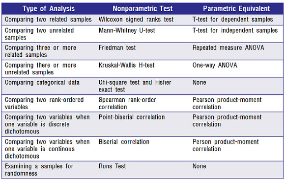
(3) 모수 VS 비모수 통계

  • 통계 분석 방법은 매우 중요하다. 일종의 가이드라인이기 때문이다.
  • 모수 통계는 기본적으로 평균들의 차이를 파악해야 하기 때문에 연속형 자료형이 필요하다. 또한, 이러한 자료는 대개 정규분포라는 형태로 잘 포장되어야 하지만, 실상은 그렇지 않다.
  • 이러한 경우 비모수적 검정을 실시한다.
    • 비모수적 검정의 기본 조건은 모수 통계를 할 수 없는 상황이 생기면, 보다 완화된 조건으로 해석하는 것이 옳은 방법이다. (가정을 무시하는 것은 아니다!)
  • 비모수 검정에는 크게 윌콕슨 순위합 검정, 윌콕슨 부호순위 검정, 프리드먼 검정, 그리고 크러스컬-월리스 검정 등이 사용된다.
  • 정규성 검정에 따른 모수와 비모수 검정 방법은 다음과 같다.
  • T검정
    • 모수적 방법: 독립표본 T검정, 대응표본 T검정
    • 비모수적 방법: 윌콕슨(Wilcoxon) 검정, 맨-휘트니(Mann-Whitney) 검정
  • 분산분석
    • 모수적 방법: 일원 배치 분산분석
    • 비모수적 방법: 크루스칼-윌리스(Kruskal-Wallis)검정
  • 관계분석
    • 모수적 방법: 피어슨의 상관분석
    • 비모수적 방법: 스피어만의 로 상관분석
  • 삼성카드의 데이터는 일반적인 모수적 방법으로는 통계검정을 하기에는 어려움이 있다. 즉, 비모수 통계에 대한 기본적인 숙지가 필요하며, 파이썬에서 비모수 통계 소스코드 예제는 추후에 다시 정리한다.

범주형 데이터 시각화를 통한 EDA 보고서

  • 범주형 데이터 시각화를 진행한다.
  • matplotlib 모듈을 활용한다.

(1) Label이 있는 그룹 막대 그래프 (예제)

  • 막대그래프를 그린, 라벨링까지 적용해본다.
  • 먼저 공식 튜토리얼에 있는 것을 확인해본다.
import matplotlib
import matplotlib.pyplot as plt
import numpy as np


labels = ['G1', 'G2', 'G3', 'G4', 'G5']
men_means = [20, 34, 30, 35, 27]
women_means = [25, 32, 34, 20, 25]

x = np.arange(len(labels)) # x축 라벨의 위치를 말한다. 
y_labels = [0, 5, 10, 15, 20, 25, 30, 35] # y축 라벨의 위치를 말한다.
width = 0.35 # 막대의 너비를 말한다. 

fig, ax = plt.subplots() # 객체를 설정하는 것이다.
rects1 = ax.bar(x - width/2, men_means, width, label = "Men")
rects2 = ax.bar(x + width/2, women_means, width, label = "Women")

png

머신러닝 지도학습 - 선형회귀

I. 개요

  • 머신러닝으로서 회귀 모형에 대해 숙지한다.
  • 회귀 모형의 기본적인 개념과 평가 지표에 대해 숙지한다.

II. 회귀 모형 개요

  • 회귀(Regression)은 통계 이론 중 가장 기본이다.
  • 회귀의 기원은 영국의 통계학자 갈톤(Galton)이 수행한 연구에서 유래한다.

  • 부모와 자식 간의 키의 상관관계를 분석하였는데, 키가 작은 가정과 키가 큰 가정을 살펴본 결과, 무한정 작아지지도 않고, 무한정 커지지 않아 일정한 평균으로 회귀하려는 자연적 법칙을 발견했다는 것이 기원이다.

(1) 회귀식의 개요

  • 회귀는 1차 방정식이다.
    • 지역, 방의 면적, 크기 등 여러 개의 독립변수에 따라 아파트 가격이라는 종속변수가 어떠한 관계를 나타내는지를 예측하고 모델링하는 것
    • 즉, 수치를 예측할 때 사용한다.

$$ Y = W_{1}\times W_{1} + W_{2}\times W_{2} + W_{3}\times W_{3} + \cdot \cdot \cdot + W_{n}\times W_{n} $$

입문자를 위한 머신러닝 개요

개요

  • 캐글 데이터를 불러오는 방법에 대해 숙지한다.
  • 머신러닝의 일반적인 내용에 대해 숙지한다.

I. 사전 준비작업

  • Kaggle API 설치 및 연동해서 GCP에 데이터를 적재하는 것까지 진행한다.

(1) Kaggle API 설치

  • 구글 코랩에서 API를 불러오려면 다음 소스코드를 실행한다.
!pip install kaggle
Requirement already satisfied: kaggle in /usr/local/lib/python3.6/dist-packages (1.5.6)
Requirement already satisfied: urllib3<1.25,>=1.21.1 in /usr/local/lib/python3.6/dist-packages (from kaggle) (1.24.3)
Requirement already satisfied: certifi in /usr/local/lib/python3.6/dist-packages (from kaggle) (2020.6.20)
Requirement already satisfied: tqdm in /usr/local/lib/python3.6/dist-packages (from kaggle) (4.41.1)
Requirement already satisfied: requests in /usr/local/lib/python3.6/dist-packages (from kaggle) (2.23.0)
Requirement already satisfied: python-slugify in /usr/local/lib/python3.6/dist-packages (from kaggle) (4.0.1)
Requirement already satisfied: python-dateutil in /usr/local/lib/python3.6/dist-packages (from kaggle) (2.8.1)
Requirement already satisfied: six>=1.10 in /usr/local/lib/python3.6/dist-packages (from kaggle) (1.12.0)
Requirement already satisfied: idna<3,>=2.5 in /usr/local/lib/python3.6/dist-packages (from requests->kaggle) (2.10)
Requirement already satisfied: chardet<4,>=3.0.2 in /usr/local/lib/python3.6/dist-packages (from requests->kaggle) (3.0.4)
Requirement already satisfied: text-unidecode>=1.3 in /usr/local/lib/python3.6/dist-packages (from python-slugify->kaggle) (1.3)

(2) Kaggle Token 다운로드

  • Kaggle에서 API Token을 다운로드 받는다.
  • [Kaggle]-[My Account]-[API]-[Create New API Token]을 누르면 kaggle.json 파일이 다운로드 된다.
  • 이 파일을 바탕화면에 옮긴 뒤, 아래 코드를 실행 시킨다.
from google.colab import files
uploaded = files.upload()
for fn in uploaded.keys():
  print('uploaded file "{name}" with length {length} bytes'.format(
      name=fn, length=len(uploaded[fn])))
  
# kaggle.json을 아래 폴더로 옮긴 뒤, file을 사용할 수 있도록 권한을 부여한다. 
!mkdir -p ~/.kaggle/ && mv kaggle.json ~/.kaggle/ && chmod 600 ~/.kaggle/kaggle.json

Upload widget is only available when the cell has been executed in the current browser session. Please rerun this cell to enable.

삼성카드 대회 Track-2 데이터 고려 사항 (1)

대회 소개

  • 삼성카드 데이터분석 공모전이 시행되고 있다.
    • 대회에 처음 참여하는 아시아경제-수강생들을 위해 일종의 가이드라인으로 제안하고자 한다.
  • 본 포스트에서는 기본적인 내용만 전달하고자 함을 밝힌다.
    • Track2 과정은 마케팅 전략 제안이 중요하다!

환경 세팅

  • 먼저, 데이터가 모두 한글로 구성이 되어 있기 때문에 한글파일 설정부터 진행한다.
  • 한글파일 설정이 완료되면 구글 드라이브와 연동한다.
  • 데이터 시각화를 진행한다.
%config InlineBackend.figure_format = 'retina'
!sudo apt-get -qq -y install fonts-nanum
The following package was automatically installed and is no longer required:
  libnvidia-common-440
Use 'apt autoremove' to remove it.
The following NEW packages will be installed:
  fonts-nanum
0 upgraded, 1 newly installed, 0 to remove and 39 not upgraded.
Need to get 9,604 kB of archives.
After this operation, 29.5 MB of additional disk space will be used.
Selecting previously unselected package fonts-nanum.
(Reading database ... 144579 files and directories currently installed.)
Preparing to unpack .../fonts-nanum_20170925-1_all.deb ...
Unpacking fonts-nanum (20170925-1) ...
Setting up fonts-nanum (20170925-1) ...
Processing triggers for fontconfig (2.12.6-0ubuntu2) ...
from pandas.plotting import register_matplotlib_converters
import seaborn as sns
import pandas as pd
import matplotlib.pyplot as plt
import matplotlib as mpl
import matplotlib.font_manager as fm
fontpath = '/usr/share/fonts/truetype/nanum/NanumBarunGothic.ttf'
font = fm.FontProperties(fname=fontpath, size=9)
plt.rc('font', family='NanumBarunGothic') 
plt.rcParams["figure.figsize"] = (20, 10)
register_matplotlib_converters()
mpl.font_manager._rebuild()
mpl.pyplot.rc('font', family='NanumGothic')
fm._rebuild()
  • 여기까지 실행하였으면 구글 코랩에서 런타임-런타임 다시 시작을 클릭한다.

구글 드라이브 연동

  • 이제 구글 드라이브를 연동한다.
# Mount Google Drive
from google.colab import drive # import drive from google colab

ROOT = "/content/drive"     # default location for the drive
print(ROOT)                 # print content of ROOT (Optional)
drive.mount(ROOT, force_remount=True)           # we mount the google drive at /content/drive
/content/drive
Go to this URL in a browser: https://accounts.google.com/o/oauth2/auth?client_id=947318989803-6bn6qk8qdgf4n4g3pfee6491hc0brc4i.apps.googleusercontent.com&redirect_uri=urn%3aietf%3awg%3aoauth%3a2.0%3aoob&scope=email%20https%3a%2f%2fwww.googleapis.com%2fauth%2fdocs.test%20https%3a%2f%2fwww.googleapis.com%2fauth%2fdrive%20https%3a%2f%2fwww.googleapis.com%2fauth%2fdrive.photos.readonly%20https%3a%2f%2fwww.googleapis.com%2fauth%2fpeopleapi.readonly&response_type=code

Enter your authorization code:
··········
Mounted at /content/drive
# import join used to join ROOT path and MY_GOOGLE_DRIVE_PATH
from os.path import join  

# path to your project on Google Drive
MY_GOOGLE_DRIVE_PATH = 'My Drive/Colab Notebooks/samsung/datasets'

PROJECT_PATH = join(ROOT, MY_GOOGLE_DRIVE_PATH)
%cd "{PROJECT_PATH}"
/content/drive/My Drive/Colab Notebooks/samsung/datasets
%ls
'[기타] SCDC_공모전 테이블 설명.xlsx'  '[Track1_데이터4] variable_dtype.xlsx'
'[Track1_데이터1] mrc_info.csv'        '[Track2_데이터1] trend_w_demo.csv'
'[Track1_데이터2] samp_train.csv'      '[Track2_데이터2] 업종_예시.xlsx'
'[Track1_데이터3] samp_cst_feat.csv'

데이터 불러오기

  • 패키지를 불러오기 위해 pandas 패키지를 활용하여 [Track2_데이터1] 데이터를 불러온다.
  • 파일을 불러 올 때, encoding="EUC-KR"를 설정해서 가져온다.
import pandas as pd

trend_w_demo = pd.read_csv('[Track2_데이터1] trend_w_demo.csv', encoding="EUC-KR")
trend_w_demo.head()
YMCategory성별구분연령대기혼스코어유아자녀스코어초등학생자녀스코어중고생자녀스코어대학생자녀스코어전업주부스코어
0202005할인점0Fhighlowhighmidlowlow
1202005취미0Bhighlowmidmidlowlow
2202005오픈마켓/소셜1Dmidmidmidmidlowmid
3202005뷰티0Dmidmidmidmidlowlow
4202005오픈마켓/소셜0Ghighlowmidmidmidlow
trend_w_demo['기혼스코어'].value_counts()
high    314088
mid     107368
low      30582
Name: 기혼스코어, dtype: int64
  • 위 데이터는 전형적으로 범주형으로 구성이 되어 있다.
  • 위 변수에서 고려할 것이 있다.
    • Category, 성별구분, 연령대는 명목형 변수인데 반해
    • 기혼스코어:전업주부스코어의 경우는 확률이다.
  • 각 스코어의 확률에 대한 정의는 다음과 같다.
    • 기혼스코어 : 카드 이용 고객이 기혼일 확률
    • 유아자녀스코어 : 카드 이용 고객이에게 유아자녀가 있을 확률
    • 초등학생자녀스코어 : 카드 이용 고객이에게 초등학생 자녀가 있을 확률
    • 중고생자녀스코어 : 카드 이용 고객이에게 중고생 자녀가 있을 확률
    • 대학생자녀스코어 : 카드 이용 고객이에게 대학생 자녀가 있을 확률
    • 전업주부스코어 : 카드 이용 고객이 전업주부일 확률
  • 위 스코어의 데이터는 단순히 명목형이라고 보기는 어렵다. 즉, 순위(서열)형 척도/등간척도로 봐야 할 것이다.

측정척도의 유형과 내용

  • 명목척도: 범주형 데이터로 측정된 측정대상을 단순히 범주로 분류하기 위한 목적으로 숫자를 부여한 척도(수학적 가감승제 계산 안 됨)
    • 예시 - 성별, 종교, 직업, 혈액형
  • 순위(서열)척도: 범주형 데이터로 명목척도의 기능뿐 아니라 각 범주 간의 대소관계, 순위(서열성)에 관하여 숫자를 부여한 척도(수학적 가감승제 계산 안 됨)
    • 예시 - 학력, 건강상태 등
  • 등간척도: 연속형 데이터로 절대적 영점(absoulute zero)이 없으며 대상이 갖는 양적인 정도의 차이에 따라 등간격으로 숫자를 부여한 척도(수학적 가감승제 계산 안 됨)
    • 예시 - 온도, 만족도(리커트척도), 충성도(리커트척도), 물가지수, 생산지수 등
  • 비율척도: 연속형 데이터로 절대적 영점이 존재하며, 비율계산이 가능한 숫자를 부여한 척도(수학적 가감승제 계산 가능)
    • 매출액, 무게, 가격, 소득, 길이, 부피 등)

(1) 척도와 분석 간의 관계

  • 척도와 분석 간의 관계에 관한 표는 아래와 같다 (신건권, 2018).
독립변수종속변수분석방법
범주형 변수(명목, 서열)범주형 변수(명목, 서열)교차분석, 카이제곱
범주형 변수(명목, 서열)연속형 변수(등간, 비율)t-검증, 분산분석, 다변량분산분석
연속형 변수(등간, 비율)범주형 변수(명목, 서열)판별분석, 군집분석, 로지스틱회귀분석
연속형 변수(등간, 비율)연속형 변수(등간, 비율)상관분석, 회귀분석, 경로분석/구조방정식모델링분석
  • 즉, 위 표를 기준으로 삼성카드를 매우 단순하게 본다면 교차분석 외에는 쓸만한 분석방법이 떠오르지 않는다.
  • 그러나, 연도, Category, 성별구분, 연령대를 제외하고는 나머지 변수들을 서열 또는 등간으로 본다면 조금 더 다양한 분석 방법이 생길 수 있다.

(2) 시각화 방법

  • 순위 및 서열척도를 다루는 데이터에 대한 시각화는 주로 다음과 같다.

(3) 모수 VS 비모수 통계

  • 통계 분석 방법은 매우 중요하다. 일종의 가이드라인이기 때문이다.
  • 모수 통계는 기본적으로 평균들의 차이를 파악해야 하기 때문에 연속형 자료형이 필요하다. 또한, 이러한 자료는 대개 정규분포라는 형태로 잘 포장되어야 하지만, 실상은 그렇지 않다.
  • 이러한 경우 비모수적 검정을 실시한다.
    • 비모수적 검정의 기본 조건은 모수 통계를 할 수 없는 상황이 생기면, 보다 완화된 조건으로 해석하는 것이 옳은 방법이다. (가정을 무시하는 것은 아니다!)
  • 비모수 검정에는 크게 윌콕슨 순위합 검정, 윌콕슨 부호순위 검정, 프리드먼 검정, 그리고 크러스컬-월리스 검정 등이 사용된다.
  • 정규성 검정에 따른 모수와 비모수 검정 방법은 다음과 같다.
  • T검정
    • 모수적 방법: 독립표본 T검정, 대응표본 T검정
    • 비모수적 방법: 윌콕슨(Wilcoxon) 검정, 맨-휘트니(Mann-Whitney) 검정
  • 분산분석
    • 모수적 방법: 일원 배치 분산분석
    • 비모수적 방법: 크루스칼-윌리스(Kruskal-Wallis)검정
  • 관계분석
    • 모수적 방법: 피어슨의 상관분석
    • 비모수적 방법: 스피어만의 로 상관분석
  • 삼성카드의 데이터는 일반적인 모수적 방법으로는 통계검정을 하기에는 어려움이 있다. 즉, 비모수 통계에 대한 기본적인 숙지가 필요하며, 파이썬에서 비모수 통계 소스코드 예제는 추후에 다시 정리한다.

Reference

DataFrame의 변수 추가 및 삭제

강의 홍보

데이터 개요

  • German Credit Card를 활용하여 데이터를 가공하도록 한다.
    • 데이터셋에 대한 설명은 Kaggle에서 확인한다.
import pandas as pd
print(pd.__version__)
1.0.5
url = 'https://raw.githubusercontent.com/chloevan/kaggle2portpolio/master/datasets/german_credit_data.csv'
german_credit = pd.read_csv(url)
german_credit.head(3)
Unnamed: 0AgeSexJobHousingSaving accountsChecking accountCredit amountDurationPurpose
0067male2ownNaNlittle11696radio/TV
1122female2ownlittlemoderate595148radio/TV
2249male1ownlittleNaN209612education
  • Pandas DataFrameIndex와 나머지 열로 구성이 되어 있다.
  • 데이터의 행과 크기를 알아보는 가장 좋은 방법은 DataFrame객체의 shape변수를 이용하는 것이다.
print('DataFrame 크기: ', german_credit.shape)
DataFrame 크기:  (1000, 10)
  • 생성된 DataFrame 객체인 german_credit은 10개의 칼럼으로 이루어져 있다.
  • 이번에는 describe() 함수를 활용하여 개략적인 분포도를 확인한다.
german_credit.describe()
Unnamed: 0AgeJobCredit amountDuration
count1000.0000001000.0000001000.0000001000.0000001000.000000
mean499.50000035.5460001.9040003271.25800020.903000
std288.81943611.3754690.6536142822.73687612.058814
min0.00000019.0000000.000000250.0000004.000000
25%249.75000027.0000002.0000001365.50000012.000000
50%499.50000033.0000002.0000002319.50000018.000000
75%749.25000042.0000002.0000003972.25000024.000000
max999.00000075.0000003.00000018424.00000072.000000
german_credit['Sex'].value_counts()
male      690
female    310
Name: Sex, dtype: int64
  • Sex의 반환 결과는 1이 700개, 0이 300개로 확인할 수 있다.
  • 이 때 value_counts()는 많은 건수 순서로 정렬되어 값을 반환한다.

새로운 변수 추가

  • 기존 데이터에서 변수를 추가하고 삭제하는 것을 진행해본다.
  • 이러한 과정을 보통 도출변수로 표현되기도 한다.
german_credit['Age+100'] = german_credit['Age'] + 100
german_credit.shape
(1000, 11)

(1) 수치형 조건에 따른 변수 추가

  • 수치형 변수의 특성에 따라 새로운 변수를 추가한다.
  • Age를 기준으로 크게 ">50"<=50이하로 구분한다.
  • 그러기 위해서는 각 조건이 맞는지를 확인하는 if 조건과 반복 수행을 위한 for-loop 조건이 필요하다.
# 빈 리스트 객체 생성
age_group = []

for age in german_credit['Age']:
  if age > 50:
    age_group.append('>50')
  else:
    age_group.append('<=50')

(age_group[0:3])
['>50', '<=50', '<=50']
  • 출력된 결과물은 위와 같은 형태로 저장된 것을 확인할 수 있다.
  • age_group에 저장된 리스트 값을 새로운 변수로 추가한다.
german_credit['Age_group'] = age_group
german_credit['Age_group'].value_counts()
<=50    887
>50     113
Name: Age_group, dtype: int64

(2) 문자형 조건에 따른 변수 추가

  • 이번에는 특정문자열의 존재 유무에 따라 새로운 column is_own을 추가한다.
german_credit['Housing'].value_counts()
own     713
rent    179
free    108
Name: Housing, dtype: int64
  • 위 데이터에서 own인 경우는 True 그렇지 않은 경우는 False로 저장한다.
  • np.where을 사용하면 if처럼 매우 쉽게 사용이 가능하다.
import numpy as np 
german_credit['is_own'] = np.where(german_credit['Housing'] == "own", True, False)
german_credit['is_own'].value_counts()
True     713
False    287
Name: is_own, dtype: int64

변수 삭제

  • 이렇게 생성된 변수를 삭제하도록 한다.
  • 이 때, 가장 많이 사용되는 함수는 drop() 메서드를 이용한다.
  • 함수 사용 시, 주의해야 하는 것 중 하나는 axis 0은 행의 방향, axis 1은 열의 방향 축으로 움직인다.
    • 즉, drop()함수를 사용 시에는 axis 1를 같이 입력한다.
german_credit = german_credit.drop('Age+100', axis = 1)
german_credit.shape
(1000, 12)
  • 이번에는 두개의 변수를 추가한 뒤, 한꺼번에 삭제하는 예제를 실습해본다.
german_credit['age+10'] = german_credit['Age'] + 10
german_credit['age+20'] = german_credit['Age'] + 20
german_credit.shape
(1000, 14)
  • 이제 새로 추가된 변수 2개를 삭제 한다.
german_credit = german_credit.drop(['age+10', 'age+20'], axis = 1)
german_credit.shape
(1000, 12)
  • 이렇게 두개 이상의 변수를 삭제할 때는 list를 활용해서 삭제가 가능하다.

정리

  • DataFrame에서 간단하게 변수를 추가 및 삭제하는 방법에 대해 배웠다.
    • 수치형 변수를 활용한 변수 추가, 문자형 변수를 활용한 변수 추가의 기본적인 내용을 숙지한다.
  • 변수를 삭제할 때는 drop()메서드를 사용하는 데, 행을 삭제할 때는 axis = 0, 열을 삭제할 때는 axis = 1 활용한다.