강의 홍보
통계분석을 활용한 문제해결 과정
- 비즈니스에서 통계는 그저 툴이다.
- 통계를 몰라도 물건을 파는데 전혀 문제가 없다.
- 통계는 객관적인 근거를 확보하여 유효한 의사결정을 내리기 위한 그저 도구
(Tool) 이다. - 따라서, 마케팅이나 CRM과 같은 경영이슈에서도 통계는 문제해결을 이한 체계적인 절차를 제공한다.
- 문제정의
- 가설수립 및 분석방법 설정
- 유의수준 및 임계치 설정
- 분석 및 검정 통계량 산출
- 결과 해석 및 가설 검증
예제를 활용한 통계분석 예제
- 데이터 분석에서 가장 자주 사용되는 통계 기법 중의 하나는
t-검정이다. - 처음
t-검정을 배울 때는 비슷한 용어들이 많아서 혼동이 오기도 했다.z-검정, t-검정, 분산분석- 이 중 2개 이하의 집단에서 평균을 비교하는 것은
z-검정, t-검정은 사실 동일한 분석방법이다. - 그러나, 실무에서는
t-검정을 자주 사용한다 (모집단의 분산을 알 수 있는 방법이 없다, 이는 자세히 한번 얘기하도록 하겠다)
(1) 문제 정의
- 이제 부터 상상의 나래를 펼쳐보자.
- 이제 온라인 쇼핑몰을 운영하는 사장이다.
- 마케팅 부서에서는 콜센터를 통해 접수된 클레임 고객에 대한
타겟마케팅을 기획한다. 클레임 고객은 상대적으로 매장을 찾는 횟수가 적어져 이탈위험도가 높을 것이라고 예상되기 때문이다.
(2) 가설설정 및 분석방법
- 이제 가설 설정을 한다.
t검정을 실시할 때는 보통의 경우 평균의 차이는 없는 것으로 정한다.- $H_{0}$(귀무가설) =
A쇼핑 클레임 고객들과 비클레임 고객들의 방문 횟수 차이는 없다. - $H_{1}$(연구가설) =
A쇼핑 클레임 고객들과 비클레임 고객들의 방문횟수 차이는 있다.
- 즉, 두 그룹간의
평균 비교이다.
(3) 데이터 수집 및 분석방법
- 독립표본
t-검정을 수행하기 위해서는 평균과 등분산 여부, 그리고 t-value(검정 통계량)과 p-value(유의확률)을 출력한다.- 가장 중요한 것은 두 그룹간의 분산이 동일한지 확인할 필요가 있다.
- 먼저 데이터를 불러온다.
# Mount Google Drive
from google.colab import drive # import drive from google colab

ROOT = "/content/drive"     # default location for the drive
print(ROOT)                 # print content of ROOT (Optional)
drive.mount(ROOT)           # we mount the google drive at /content/drive
/content/drive
Drive already mounted at /content/drive; to attempt to forcibly remount, call drive.mount("/content/drive", force_remount=True).
# import join used to join ROOT path and MY_GOOGLE_DRIVE_PATH
from os.path import join

# path to your project on Google Drive
MY_GOOGLE_DRIVE_PATH = 'My Drive/Colab Notebooks/inflearn/Python/Kaggle_Edu/05_statistics'

PROJECT_PATH = join(ROOT, MY_GOOGLE_DRIVE_PATH)
print(PROJECT_PATH)
/content/drive/My Drive/Colab Notebooks/inflearn/Python/Kaggle_Edu/05_statistics
/content/drive/My Drive/Colab Notebooks/inflearn/Python/Kaggle_Edu/05_statistics
import pandas as pd
data = pd.read_csv('python_stat/Ashopping.csv', sep=",", encoding='CP949')
data.head()
| 고객ID | 이탈여부 | 총_매출액 | 방문빈도 | 1회_평균매출액 | 할인권_사용 횟수 | 총_할인_금액 | 고객등급 | 구매유형 | 클레임접수여부 | 구매_카테고리_수 | 거주지역 | 성별 | 고객_나이대 | 거래기간 | 할인민감여부 | 멤버쉽_프로그램_가입전_만족도 | 멤버쉽_프로그램_가입후_만족도 | Recency | Frequency | Monetary | 상품_만족도 | 매장_만족도 | 서비스_만족도 | 상품_품질 | 상품_다양성 | 가격_적절성 | 상품_진열_위치 | 상품_설명_표시 | 매장_청결성 | 공간_편의성 | 시야_확보성 | 음향_적절성 | 안내_표지판_설명 | 친절성 | 신속성 | 책임성 | 정확성 | 전문성 |
|---|
| 0 | 1 | 0 | 4007080 | 17 | 235711 | 1 | 5445 | 1 | 4 | 0 | 6 | 6 | 1 | 4 | 1079 | 0 | 5 | 7 | 7 | 3 | 4 | 6 | 5 | 6 | 7 | 7 | 6 | 7.0 | 6.0 | 6 | 7 | 6 | 6 | 6 | 6 | 6 | 6 | 6 | 6 |
|---|
| 1 | 2 | 1 | 3168400 | 14 | 226314 | 22 | 350995 | 2 | 4 | 0 | 4 | 4 | 1 | 1 | 537 | 0 | 2 | 3 | 2 | 3 | 3 | 2 | 5 | 4 | 6 | 7 | 6 | 6.0 | NaN | 7 | 7 | 6 | 6 | 6 | 5 | 3 | 6 | 6 | 6 |
|---|
| 2 | 3 | 0 | 2680780 | 18 | 148932 | 6 | 186045 | 1 | 4 | 1 | 6 | 6 | 1 | 6 | 1080 | 0 | 6 | 6 | 7 | 3 | 2 | 4 | 6 | 7 | 6 | 7 | 6 | 7.0 | NaN | 6 | 6 | 6 | 6 | 6 | 7 | 7 | 6 | 6 | 7 |
|---|
| 3 | 4 | 0 | 5946600 | 17 | 349800 | 1 | 5195 | 1 | 4 | 1 | 5 | 5 | 1 | 6 | 1019 | 0 | 3 | 5 | 7 | 3 | 5 | 3 | 5 | 5 | 6 | 6 | 6 | 5.0 | 6.0 | 6 | 6 | 5 | 6 | 6 | 6 | 6 | 6 | 5 | 6 |
|---|
| 4 | 5 | 0 | 13745950 | 73 | 188301 | 9 | 246350 | 1 | 2 | 0 | 6 | 6 | 0 | 6 | 1086 | 0 | 5 | 6 | 7 | 6 | 7 | 5 | 6 | 6 | 5 | 6 | 6 | 5.0 | 6.0 | 5 | 6 | 6 | 6 | 5 | 5 | 6 | 6 | 5 | 6 |
|---|
- 데이터를 확인했다면, 이제, 클레임 접수여부에 따라 클레임이 없는 (0)고객과, 클레임이 있는 고객(1) 객체에 저장후 두 그룹의 방문빈도를 추출한다.
- 우선 클레임이 없는 고객을 뽑자.
import numpy as np
no_claim = data[data.클레임접수여부 == 0]
no_claim_array = np.array(no_claim.방문빈도)
no_claim_array
array([ 17,  14,  73,  26,   6,  17,  19,  88,  39,  12,  27,  21,  56,
        16,  21,  28,  17,  15,  48,  42,  33,   9,  32,  15,  23,  24,
        18,  18,  38,  15,  16,  36,   8,  33,  41,  34,  12,  56,  60,
        27,  10,  39,  48,  24,   8,   7,  25,  19,  33,  22,  30,   9,
        80,  18,  15,  50,  71,  15,  66,  41,  18,   5,  78,  30,  14,
        10,  54,  21,  43,  33,  24,  21,  13,  25,  37,  25,  47,  60,
        21,  23,  18,  26,  28,  31,  58,  88,  19,  38,  37,  20,  33,
        18,  15,   7,  29,  30,   6,  16,  10,  23,  10,  14,  18,  11,
        15,  14,  90,   9,   9,   5,  15,  11,  33,   9,  20,   6,  42,
        17,  78,   9,  20,  37,  14,  17,  25,  52,  19,   9,  26,  16,
        49,  32,  24,  40,  44,  13,  16,  25,  16,  47,  27,   9,  15,
         5,  26,  34,  39,  18,  28,  16,  32,  81,  15,  41,   9,  10,
         9,   8,  56,  12,  65,  10,  45,  60,  22,  52,  15,  61,  18,
        12,  23,  93,  28,  12,  39, 103,  11,  28,   6,  35,   6,  86,
        17, 185,  16,  37,  21,  22,  50,  37,  14,  15,  28,  14,  11,
        31,  31,  59,  26,  20,  29,  23,  11,  29,  11, 108,   6,  37,
        29,  12,  11,  10,  18,  36,  73,  18,  22,  14,  22,  13,  31,
        15,  31,  25,  52,  10,  35,   9,   9,   5,  27,  12,  79,  21,
         8,  11,  64,  22,  60,  31,  15,  48,  18,   8,  31,  14,  46,
       102,  10,  34,   4,  23,  43,  45,   9,  18,  26,  12,   8,  81,
        51,  14,  28,  18,  24,  28,  15,  29,   8,   5,  17,  16,  28,
        36,  27,  11,  10,  20,  13,  54,  23,  14,  27,  13,  38,  38,
        79,  27,  97,   8,  10,  41,   6,  19,  16,  21,  46,  23,  39,
        38,  19,   7,   6,  33,  61,  15,  10, 114,  71,  33,  25,  79,
        13,  29,  34,  30,  19,  23,  40,  15,  17,   8,   3,   7,  21,
         9,  40,  46,  24,  73,  38,  56,  13,  13,  30,  46,   6,  30,
        19,   5,  20,  23,   7,  20,  26,  15,  58,  15,  11,  31,  17,
        10,  14,  20,  10,  50,  21,  37,  30,   6,  16,  23,  21, 102,
        26,  43,   8,  15,  10,  14,  71,  60,  45,  25,  49,  50,   9,
        18,  23,  29, 106,  35,  22,  12, 203,  12,  17,  14,  39,  11,
        19,  29,  22,  21,   9,  22,  11,  21,  58,  10,   5,  16,  39,
        13,  33,  13,  14,  13,  18,  42,  11,  29,  28,  35,   9,  21,
        26,  17,  24,   5,  23,  71,  22,  20,  20,   7,  14,  12,  10,
        16,  18,  30,  25,  22,  15,  18,  43,  33,  46,  14,  12,  24,
        23,  18,  23,   9,  13,  17,  22,   7,  18,  15,  39,  22,  22,
        22,   9,  15,  36,  24,  32,  38, 109,  28,  23,  20,  76,  43,
        25,   5,  46,  10,  22,  18,  30,  75,  34,  11,  17,  43,  39,
        84,  42,  41,  26,  32,  31,  37,  15,  50,  22,  19,   6,  19,
        11,   7,  25,  63,  21,  16,  67,  27,   5,  32,  31, 114,  20,
        21,  14,  80,  19,  14,  32,   4,  15,  37,  24,  14,  11,  10,
        20,  30,  10,  19,   6,  26,  26,   9,   4,  66,  16,  24,  29,
        33,  20,  19,  20,  49,  10,  15,  23])
claim = data[data.클레임접수여부 == 1]
claim_array = np.array(claim.방문빈도)
claim_array
array([ 18,  17, 109,  15,  21,   9,  12,  28,   5,  12,  12,  13,   8,
        18,  27,  34,  23,  19,  29,  10,  19,  28,  23,  30,  14,  20,
         7,  14,  32,  32,  18,  17,  10,  23,  12,   9,  43,  42,   7,
        12,  73,  26,  27,  25,  29,  37,  32,  45,  34,   7,  29,  26,
        27,  33,  27,  28,   8,  45,  66,  14,  73,  24,  13,  54,  24,
        17,  29,  29,  57,  18,  17,  27,  15,  23,  11,   4,  15,  31,
        21,  21,  11,  19,  34,  41,  18,  45,  10,  72,  18,  82,  10,
        26,  17,  37,  17,   8,  26,  11,  28,  17,  12,  23,  37,  19,
         7,  20,   9,  14,  13,  36,  26,  23,  23,  16,  30,  13,  45,
        30,   6,  44,  32,  19,  20,  24,   7,  14,   7,  65,  31,   6,
        37,  91,  17,  12,  23,  61, 162,  23,  21,  12,  14,  10,  18,
        14,   4,   6,  26,  19,  27,  14,   7,  32,  11,  11,  20,   7,
         7,   7,  27,  16,  26,  10,  12,   8,  12,  25,  14,  18,  30,
        33,  86,  20,  22,  10,  34,  36,   9,  68,  28,  14,  61,   9,
        17,   6,  30,  14,  25,  32,  19,  34,  26,  17,  24,  18,  30,
        15,  15,  96,  17,  18,  19,  24,  16,   6,  27,  31,  15,  38,
        11,   7,  65,  15,   7,  23,   7,  15,  34,  17,  20,  19,  10,
        14,  19,  69,   4,  21,  13,  20,  45,  50,  58,   6,  15,  10,
        10,  19,  32,   6,  38,  36,   6,  39,  16,  20,  48,  26,  21,
        22,   7,   8,  28,   8,  31,  13,  46,  20,   8,  49,   9,  48,
        20,  25,  54,  21,   6,  30,  40,  11,  12,  28,  15,  24,  90,
        22,  15,  14,   7,  77,  39,  11,  18,  16,  55,  15,  12,  17,
        23,  15,  33,  15,  18,  28,   7,  17,  34,  27,  44,  35,  67,
        12,  54,  18,  10,  21,  28,  67,   9, 126,  23,  10,  41,  15,
        21,  21,  42,  18,  31,  13,  20,  19,  39,  26,  11,  22,  64,
         4,  27,  21,  14,  30,  25,  18,  11,  10,  70,  24,  18,  19,
        30,  30,  19, 104,  39,  92,  52,  48,  30,  79,  15,  24,  23,
        14,   8,   9,  21,  18,  11,   7,   8,  13,  21,  23,   2,  12,
        12,  52,  22,  20,   6,  22,   6,  24,  12,  18,  20,  11,  12,
        33,   8,  24,  79,  34,   8,  36,  13,  19,   5,  12,  25,  31,
        27,  17,  11,  65,  29,  18,  10,  28,  22,  12,  18,  20,  27,
        17,  20,  17,   8,  38,  18,  25,  10,   7,  18,  11,  55,   5,
        20,  11,  41,  12,  11,  26,  55,  25,   6,  35,  38,  32,  27,
        11,  10,  11,  55,  22,  12,  18,  10,  15,  32,  13,  29,   8,
        17,  83,  15,   7,   8,  11,  27,  21,  18,  15,  19,   8,  16,
        35,  15,  40,   8])
- 그 후,
stats.bartlett() 함수를 이용하여 등분산 검정을 실시한다. - 이 때, 주의해야 하는 것이 있다.
- 등분산 검정의 귀무가설과 대립가설을 다음과 같다.
- H0 : 등분산이다.
- H1 : 이분산이다(등분산이 아니다).
- 즉, 등분산 가정의 귀무가설을 채택하려면 유의확률인 0.05 > p 나와야 한다.
from scipy import stats
stats.bartlett(no_claim_array, claim_array)
BartlettResult(statistic=13.626177910965525, pvalue=0.00022305349806448475)
- 여기에서 두 고객 그룹간의 등분산 검정 결과
F값은 13.626, 유의확률은 0.05미만으로 귀무가설이 기각된다.- 즉, 두 집단의 분산은 동일하지 않은 것으로 나타났다.
- 등분산성이 나와야 하는데, 나오지 않아서 입문자들이 조금 당혹스러워 할 수 있다.
- 굳이 당황할 필요는 없다. 분산이 동일하지 않으면 동일하지 않다고 표시만 해두면 된다.
(check: equal_var)
- 이제
ttest_ind를 활용해서 구하도록 하자.
print(stats.ttest_ind(no_claim_array, claim_array, equal_var=False))
Ttest_indResult(statistic=2.595726838875684, pvalue=0.009577734932789503)
- 독립표본
t-value는 2.59이며, p-value 0.0095로 나왔다.- 이 의미는 두 그룹간의 평균 방문 빈도에 차이가 있음을 의미한다.
- 조금 더 구체적으로 구해보자.
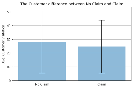
(4) 시각화
- 실제 두 그룹간의 차이를
matplotlib을 활용하여 시각화로 구현해본다. - 이 때, 각 그룹의
평균(Mean)과 표준편차(Standard Deviation)를 구한다.
# 평균 계산하기
no_claim_mean = np.mean(no_claim_array)
claim_mean = np.mean(claim_array)
print("클레임이 없는 고객의 평균 방문빈도:", no_claim_mean)
print("클레임이 있는 고객의 평균 방문빈도:", claim_mean)

# 표준편차 구하기
no_claim_std = np.std(no_claim_array)
claim_std = np.std(claim_array)
print("클레임이 없는 고객의 표준편차:", no_claim_std)
print("클레임이 있는 고객의 표준편차:", claim_std)

# 라벨 정리
viz_labels = ['No Claim', 'Claim']
x_pos = np.arange(len(viz_labels))
avg = (no_claim_mean, claim_mean)
error = [no_claim_std, claim_std]
클레임이 없는 고객의 평균 방문빈도: 28.184842883548985
클레임이 있는 고객의 평균 방문빈도: 24.736383442265794
클레임이 없는 고객의 표준편차: 22.7348095052013
클레임이 있는 고객의 표준편차: 19.234427104778828
import matplotlib.pyplot as plt

fig, ax = plt.subplots()
ax.bar(x_pos, avg,
       yerr = error,
       align='center',
       alpha=0.5,
       ecolor='black',
       capsize=10)
ax.set_ylabel('Avg. Customer Visitation')
ax.set_xticks(x_pos)
ax.set_xticklabels(viz_labels)
ax.set_title('The Customer difference between No Claim and Claim')
ax.yaxis.grid(True)

plt.tight_layout()
plt.show()