강의 홍보
공지
- 현재 책 출판 준비 중입니다.
- 구체적인 설명은 책이 출판된 이후에 요약해서 올리도록 합니다.
이전 글
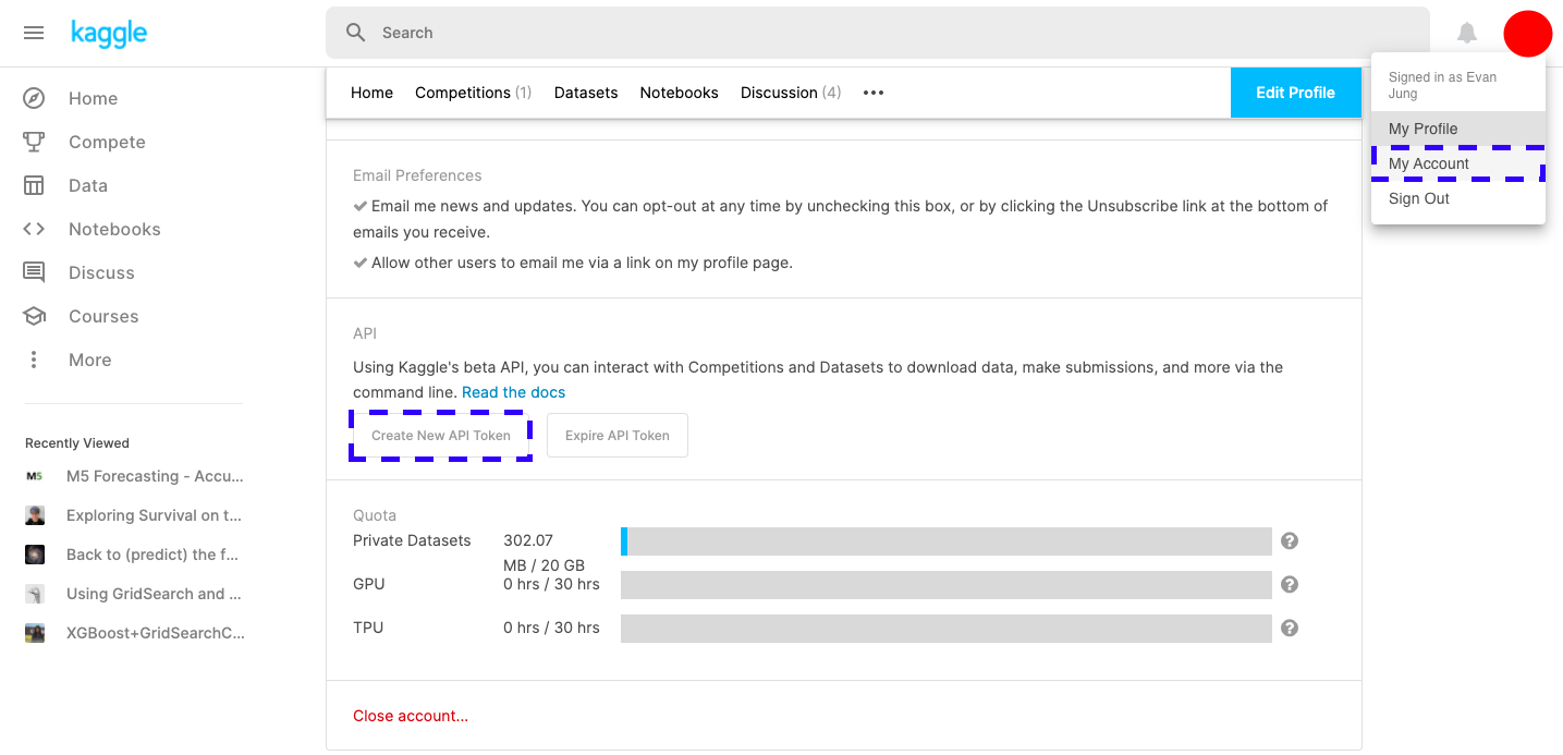
- Kaggle Feature Engineering - House Price
- 이전 글에서, Kaggle API, Feature Engineering에 대한 코드를 정리했으니, 참고하기를 바란다.
머신러닝 모형 학습 및 평가
데이터셋 분리 및 교차 검증
X = all_df.iloc[:len(y), :]
X_test = all_df.iloc[len(y):, :]
X.shape, y.shape, X_test.shape
((1458, 258), (1458,), (1459, 258))
from sklearn.model_selection import train_test_split
X_train, X_test, y_train, y_test = train_test_split(X, y, test_size = 0.25, random_state = 0)
X_train.shape, X_test.shape, y_train.shape, y_test.shape
((1093, 258), (365, 258), (1093,), (365,))
평가지표
MAE
import numpy as np

def mean_absolute_error(y_true, y_pred):

  error = 0
  for yt, yp in zip(y_true, y_pred):
    error = error + np.abs(yt-yp)

  mae = error / len(y_true)
  return mae
MSE
import numpy as np

def mean_squared_error(y_true, y_pred):

  error = 0
  for yt, yp in zip(y_true, y_pred):
    error = error + (yt - yp) ** 2

  mse = error / len(y_true)
  return mse
RMSE
import numpy as np

def root_rmse_squared_error(y_true, ypred):
  error = 0

  for yt, yp in zip(y_true, y_pred):
    error = error + (yt - yp) ** 2

  mse = error / len(y_true)
  rmse = np.round(np.sqrt(mse), 3)
  return rmse
Test1
y_true = [400, 300, 800]
y_pred = [380, 320, 777]

print("MAE:", mean_absolute_error(y_true, y_pred))
print("MSE:", mean_squared_error(y_true, y_pred))
print("RMSE:", root_rmse_squared_error(y_true, y_pred))
MAE: 21.0
MSE: 443.0
RMSE: 21.048
Test2
y_true = [400, 300, 800, 900]
y_pred = [380, 320, 777, 600]

print("MAE:", mean_absolute_error(y_true, y_pred))
print("MSE:", mean_squared_error(y_true, y_pred))
print("RMSE:", root_rmse_squared_error(y_true, y_pred))
MAE: 90.75
MSE: 22832.25
RMSE: 151.103
RMSE with Sklean
from sklearn.metrics import mean_squared_error

def rmsle(y_true, y_pred):
    return np.sqrt(mean_squared_error(y_true, y_pred))
모형 정의 및 검증 평가
from sklearn.metrics import mean_squared_error
from sklearn.model_selection import KFold, cross_val_score
from sklearn.linear_model import LinearRegression

def cv_rmse(model, n_folds=5):
    cv = KFold(n_splits=n_folds, random_state=42, shuffle=True)
    rmse_list = np.sqrt(-cross_val_score(model, X, y, scoring='neg_mean_squared_error', cv=cv))
    print('CV RMSE value list:', np.round(rmse_list, 4))
    print('CV RMSE mean value:', np.round(np.mean(rmse_list), 4))
    return (rmse_list)

n_folds = 5
rmse_scores = {}
lr_model = LinearRegression()
score = cv_rmse(lr_model, n_folds)
print("linear regression - mean: {:.4f} (std: {:.4f})".format(score.mean(), score.std()))
rmse_scores['linear regression'] = (score.mean(), score.std())
CV RMSE value list: [0.139  0.1749 0.1489 0.1102 0.1064]
CV RMSE mean value: 0.1359
linear regression - mean: 0.1359 (std: 0.0254)
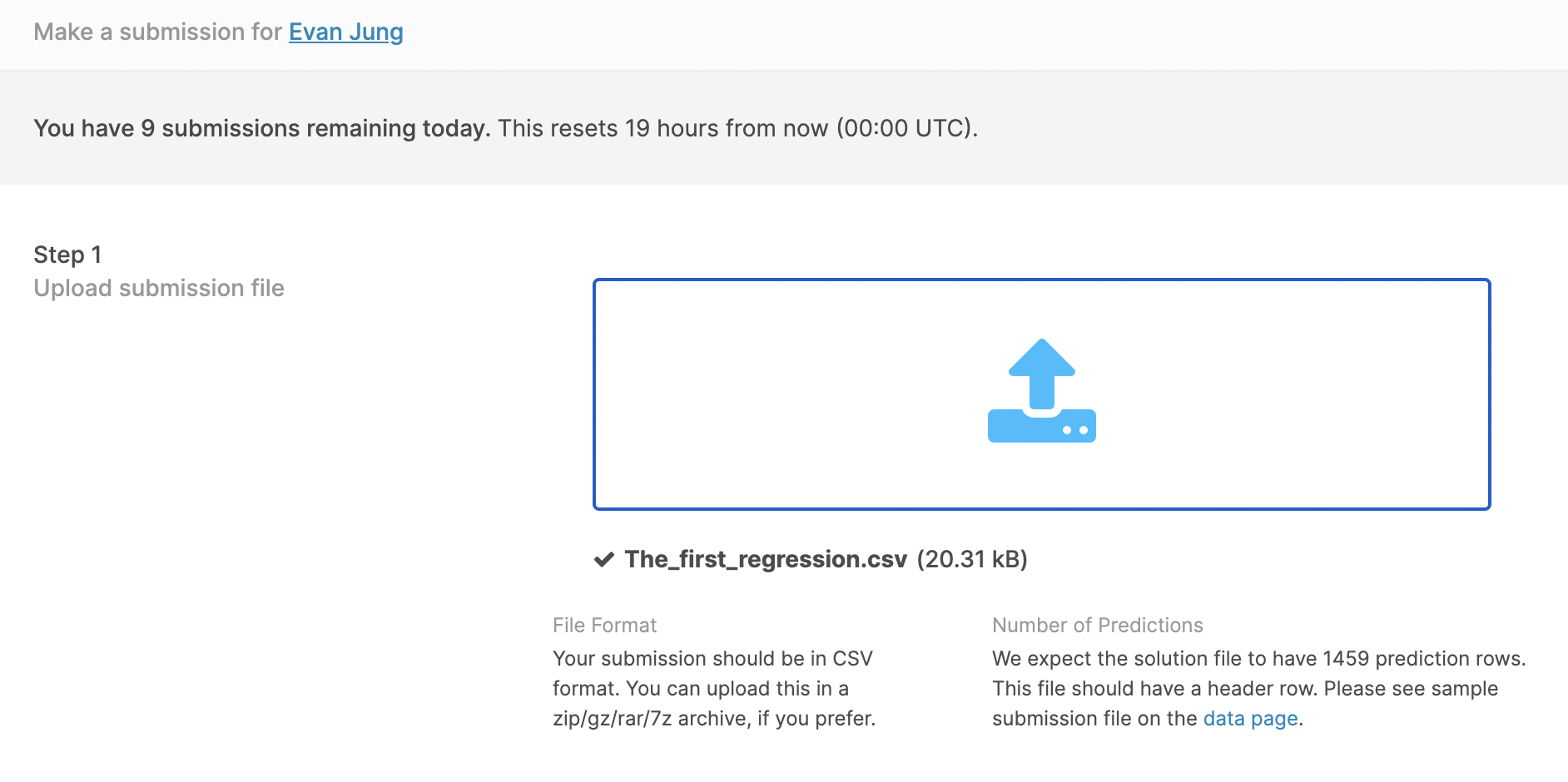
첫번째 최종 예측 값 제출
from sklearn.model_selection import cross_val_predict

X = all_df.iloc[:len(y), :]
X_test = all_df.iloc[len(y):, :]
X.shape, y.shape, X_test.shape

lr_model_fit = lr_model.fit(X, y)
final_preds = np.floor(np.expm1(lr_model_fit.predict(X_test)))
print(final_preds)
[117164. 158072. 187662. ... 173438. 115451. 219376.]
submission = pd.read_csv("sample_submission.csv")
submission.iloc[:,1] = final_preds
print(submission.head())
submission.to_csv("The_first_regression.csv", index=False)
     Id  SalePrice
0  1461   117164.0
1  1462   158072.0
2  1463   187662.0
3  1464   197265.0
4  1465   199692.0
Kaggle 업데이트